Point Estimation and Statistical Inference

• Model Fitting or Point Estimation
  • Maximum Likelihood Estimation - Frequentist Perspective
  • Why MLE?
    • $\hat{p}_{data}$ vs. $p_{model}$
    • KL Divergence and Cross Entropy
  • Empirical Risk Minimization (ERM)
    • Surrogate Loss
  • Bias-Variance Tradeoff
    • Bias of Estimator
    • Variance of Estimator
    • Bias-Variance Tradeoff
    • Underfitting and Overfitting
  • Regularization and Maximum A Posterior Estimation - Bayesian Perspective
• Frequentist Inference
  • Hypothesis Testing
  • Significance Tests and P-Values
  • Type I and Type II Error
  • Multiple Hypothesis Testing
• Bayesian Inference
• Reference

Model Fitting or Point Estimation

The process of estimating all the parameters $\mathbf{\theta}$ of a probabilistic model from a finite sample of data $\mathcal{D}$ called model fitting or training, with the optimization problem of the form

\[\hat{\theta} = \arg\min_{\theta} \mathcal{L}(\theta)\]

One common principle of parameter estimation or (point estimation) is the maximum likelihood principle.

Maximum Likelihood Estimation - Frequentist Perspective

MLE is to pick the parameters $\hat{\theta}$ that assign the highest probability to the sampled training data $\mathcal{D} = \{ (\mathbf{x}_i, y_i) \}_{i=1}^{N}$

\[\begin{aligned} \hat{\theta}_{MLE} &= \arg\max_{\theta} p(\mathcal{D} \mid \theta) \\ &= \arg\max_{\theta} \prod_{i=1}^{N} p(y_i\mid \mathbf{x}_i, \theta) \\ &= \arg\max_{\theta} \sum_{i=1}^{N} \log p(y_i\mid \mathbf{x}_i, \theta) \\ &= \arg\min_{\theta} -\sum_{i=1}^{N} \log p(y_i\mid \mathbf{x}_i, \theta) \\ &= \arg\min_{\theta} \frac{1}{N}\sum_{i=1}^{N} -\log p(y_i\mid \mathbf{x}_i, \theta) \end{aligned}\]

If the model is unconditional (unsupervised such as Gaussian Mixture Model or K-Means), the MLE becomes

\[\hat{\theta}_{MLE} = \arg\min_{\theta} -\sum_{i=1}^{N} \log p(y_i\mid \theta)\]

Why MLE?

In short, we will see that MLE is same as minimizing the KL-Divergence between the empirical distribution $\hat{p}_{data}$ defined by the training set and the model distribution $p_{model}$.

Now consider the a sef of $N$ examples $\mathcal{D}=\{y_1, \cdots, y_N \}$ drawn independently from the true but unknown data generating distribution $p_{data}(y)$. The goal of model fitting is to optimize a parametric model such that the parametric probability distribution $p_{model}(y\mid\theta)$ is similar to the true distribution. That is, $p_{model}(y \mid \theta)$ maps any $y$ to a real number estimating the true probability $p_{data}(y)$.

Dirac delta Function: $\delta(x)$ is defined such that it is zero-valued everywhere except x=0, yet integrates to 1.

As we know the PDF of a continous variable is always 0, but in some cases, we would like to specify that all of the mass in a probability distribution clusters around a single point. This can be accomplished by defining a PDF using the Dirac delta function.

For example, if we defining the PDF as

\[p(x) = \delta( x - \mu)\]

that means we have an infinitely narrow and infinitely high peak of probability mass where $x=\mu$.

Empirical Distribution: is the distribution function associated with the empirical measure of a sample:

\[\hat{p}(x) = \frac{1}{N} \sum_{i=1}^{N} \delta(x - x_i)\]

which puts probability mass $1/N$ on each of the $N$ sampled data point $x_i, \cdots, x_N$. We can view the empirical distribution formed from a dataset of training examples.

$\hat{p}_{data}$ vs. $p_{model}$

Now, we could rescale the likelihood by $1/N$ which does not affect the argmax operation and we obtains a version of the criterion that is expressed as an expectation w.r.t the empirical distribution $\hat{p}_{data}$ defined by the training data:

\[\begin{aligned} \theta_{MLE} &= \arg\max_{\theta} \sum_{i=1}^{N} \log p_{model} (y_i \mid \theta) \\ &= \arg\max_{\theta} \frac{1}{N} \sum_{i=1}^{N} \log p_{model} (y_i \mid \theta) \\ &= \arg\max_{\theta} \mathbb{E}_{y\sim \hat{p}_{data}} [\log p_{model} (y \mid \theta)] \end{aligned}\]

Now, since the true distribution $p_{data}$ is unknown, instead of minimizing the dissimilarity between the $p_{data}$ and $p_{model}$, we could try to minimize the dissimilarity between $\hat{p}_{data}$ and $p_{model}$ using KL-Divergence:

\[\begin{aligned} D_{KL}(\hat{p}_{data} \| p_{model}) &= \mathbb{E}_{y\sim \hat{p}_{data}} [ \log \hat{p}_{data}(y) - \log p_{model}(y\mid\theta) ] \\ &= \mathbb{E}_{y\sim \hat{p}_{data}} [ \log \hat{p}_{data}(y)] - \mathbb{E}_{y\sim \hat{p}_{data}} [ \log p_{model}(y\mid\theta)] \end{aligned}\]

We can see that to minimize the KL-Divergence w.r.t $\theta$ is same as minimizing the second term, that is

\[\begin{aligned} \theta_{KL} &= \arg\min_{\theta} D_{KL}(\hat{p}_{data} \| p_{model}) \\ &=\arg\min_{\theta}- \mathbb{E}_{y\sim \hat{p}_{data}} [ \log p_{model}(y\mid\theta)] \\ &=\arg\min_{\theta} \mathbb{E}_{y\sim \hat{p}_{data}} [- \log p_{model}(y\mid\theta)] \\ &= \theta_{CE}\\ &= \arg\max_{\theta} \mathbb{E}_{y\sim \hat{p}_{data}} [\log p_{model} (y \mid \theta)]\\ &= \theta_{MLE} \end{aligned}\]

where $\theta_{ce}$ denotes the parameters obtained via minimizing the cross entropy between empirical distribution and model distribution.

KL Divergence and Cross Entropy

Shannon Entropy: is defined over a distribution $p$ of a random variable $Y$:

\[\begin{aligned} H(p) &= \mathbb{E}_{p}[-\log p] \\ &= -\sum_{y\in Y} p(y) \log p(y) \end{aligned}\]

Cross Entropy: is defined over two distributions $p$ and $q$ of a random variable $Y$:

\[\begin{aligned} H(p, q) &= \mathbb{E}_{p} [-\log q]\\ &= -\sum_{y\in Y} p(y) \log q(y) \end{aligned}\]

KL Divergence: is also called relative entropy, which is defined as

\[\begin{aligned} D_{KL}(p\|q) &= \mathbb{E}_{p} [-\log \frac{q}{p}]\\ &= -\sum_{y\in Y} p(y) \log \frac{q(y)}{p(y)} \\ &= [-\sum_{y\in Y} p(y) \log q(y)] - [-\sum_{y\in Y}p(y)\log p(y)] \\ &= H(p, q) - H(p) \end{aligned}\]

Empirical Risk Minimization (ERM)

We have shown that

\[\theta_{MLE} = \arg\min_{\theta} \frac{1}{N}\sum_{i=1}^{N} -\log p(y_i\mid \mathbf{x}_i, \theta)\]

where $-\log p(y_i\mid \mathbf{x}_i, \theta)$ could be viewed as (conditional) log loss on each sampled data.

We could further generalize the MLE by replacing the (conditional) log loss term with any other loss function $\ell(y_i\mid \mathbf{x}_i, \theta)$

\[\mathcal{L}(\theta) = \frac{1}{N} \sum_{i=1}^{N} \ell(y_i\mid \mathbf{x}_i, \theta)\]

As we could see, it is the expected loss where the expectation is taken w.r.t the empirical distribution $\hat{p}_{data}$. Hence, this is also known as empirical risk minimization, which could be expressed as

\[\mathcal{L}(\theta) = \mathbb{E}_{(\mathbf{x},y)\sim \hat{p}_{data}} [\ell(\hat{y}, y)]\]

with $\hat{y} = f(\mathbf{x}; \theta)$.

However, don’t forget that our ultimate goal is to minimize the loss function where the expectation is taken across the data generating distribution $p_{data}$ rather than just over the finite training set:

\[J(\theta) = \mathbb{E}_{(\mathbf{x},y)\sim p_{data}} [\ell(\hat{y}, y)]\]

which is called expected generalization error or risk. We $\color{blue}{hope}$ that minimizing the empirical risk could result in the decrease of true risk. However, empirical risk minimization is prone to overfitting, and in many cases empirical risk minimization is not really feasible. Therefore, in practices we typically optimize an objective function that is revised based on empirical risk minimization so that it will lead to minimal of true risk.

Surrogate Loss

Consider a binary classification problem, we would like to use 0-1 loss:

0-1 Loss: is defined as follows

\[\ell_{01}(y_i\mid x_i, \theta) = \begin{cases} 0 &\quad\text{if}\quad y_i = \hat{y}_i=f(x_i \mid \theta) \\ 1 &\quad\text{if}\quad y_i \neq \hat{y}_i = f(x_i \mid \theta) \end{cases}\]

where $f(x_i\mid \theta)$ is some kind of predictor. The corresponding empirical risk is:

\[\mathcal{L}(\theta) = \frac{1}{N} \sum_{i=1}^{N} \ell_{01}(y_i\mid x_i, \theta) = \frac{1}{N} \sum_{i=1}^{N} \mathbb{I}(y_i\neq \hat{y_i})\]

Disadvantage: exactly minimizing expected 0-1 loss is typically intractable (exponential in the input dimension), even for a linear classifier.

Solution: optimize the surrogate loss.

Negative Log-Likelihood (NLL) and Log Loss: the NLL of the correct class is typically used as a surrogate for the 0-1 loss, where $\log p(y_i\mid \mathbf{x}_i; \theta)$ denotes how much the estimated label aligns with the true label and the $-\log p(y_i\mid \mathbf{x}_i; \theta)$ denotes how much the estimated label does not align with the true label which serve as the loss.

Log Loss: is used in probabilistic binary classification with true label $y\in \{-1, 1\}$. Similar to the likelihood, it produce the following distribution over labels with logistic function

\[p(y \mid \mathbf{x}; \theta) = \sigma(y\cdot(\mathbf{w}^\top\mathbf{x})) = \frac{1}{1 + e^{-y\cdot(\mathbf{w}^\top\mathbf{x})}}\]

to compute how much the predicted label aligns with the true label. Therefore, the log loss is given by

\[\ell_{ll}(y_i, \hat{y}_i) = -\log \sigma (y_i\cdot(\mathbf{w}^\top\mathbf{x}_i))\]

where $\hat{y}_i$ denote the raw output of classifier’s decision function, not the predicted class label.

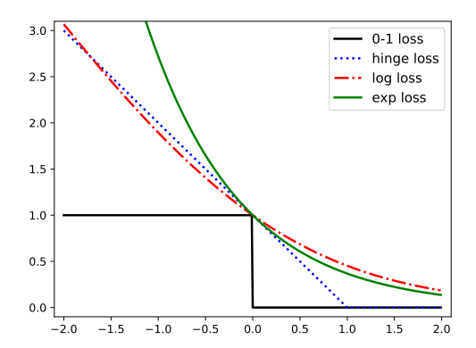
As shown in the Fig. below, minimizing the negative log likelihood on the binary classification problem is equivalent to minimizing a (fairly tight) upper bound on the empirical 0-1 loss.

Figure 1. Surrogate Loss. The horizontal axis is the$y_i\hat{y}_i$ with $y_i \in \{-1, 1\}$.

Hinge Loss: is another convex upper bound to 0-1 loss, which is defined as follows:

\[\ell_{hinge}(y_i, \hat{y}_i) = \max (0, 1-y_i\hat{y}_i)\]

where $\hat{y}_i$ denote the raw output of classifier’s decision function, not the predicted class label. It is used in SVM, and it is only piecewise differentiable.

Bias-Variance Tradeoff

Let $\{\mathbf{x}_1, \cdots, \mathbf{x}_N \}$ be a set of $N$ independent and identically distributed data points. A point estimator is any function of the data:

\[\hat{\theta}_{N} = g(\mathbf{x}_1, \cdots, \mathbf{x}_N).\]

where a good estimator is a function whose output is close to the true underlying $\theta^*$ that generated the training data.

Bias of Estimator

The bias of an estimator is defined as

\[\text{bias}(\hat{\theta}) = \mathbb{E}(\hat{\theta}_{N}) - \theta^*\]

where the expectation is over the data and $\theta^*$ is the true underlying value of $\theta$ used to define the data generating distribution.

An estimator $\hat{\theta}_N$ is said to be unbiased or asymptotically unbiased if $bias(\hat{\theta}_N) = 0$ or $\lim_{N\rightarrow \infty} \mathbb{E}(\hat{\theta}_{N}) = \theta$, respectively.

Variance of Estimator

The variance of an estimator is defined as follows:

\[\text{var}(\hat{\theta}) = \mathbb{E}[\hat{\theta}^2] - (\mathbb{E}[\hat{\theta}])^2\]

which measures how much our estimate will vary as the data changes or being resampled.

Bias-Variance Tradeoff

We could compute the mean squared error (MSE) of the estimates:

\[\begin{aligned} \mathbb{E}[(\hat{\theta}_{N}-\theta^*)^2] &= \mathbb{E}[[(\hat{\theta}-\bar{\theta}) + (\bar{\theta}-\theta^*)]^2] \\ &= \mathbb{E}[(\hat{\theta}-\bar{\theta})^2 + 2(\hat{\theta}-\bar{\theta})(\bar{\theta}-\theta^*)+(\bar{\theta}-\theta^*)^2] \\ &= \mathbb{E}[(\hat{\theta} - \bar{\theta})^2] + (\bar{\theta}-\theta^*)^2 + 2(\bar{\theta}-\theta^*)\mathbb{E}[(\hat{\theta}-\bar{\theta})] \\ &= \mathbb{E}[(\hat{\theta} - \bar{\theta})^2] + (\bar{\theta}-\theta^*)^2 + 0\\ &= var(\hat{\theta}_{N}) + bias(\hat{\theta}_N)^2 \end{aligned}\]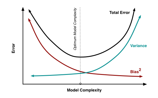

Figure 1. Bias and Variance Tradeoff on Parameter Estimation.

Underfitting and Overfitting

Two factors determine how well a model fitting algorithm is:

1. Empirical risk minimization: make the training error small.
2. Generalized risk minimization: make the gap between training and test error small.

Underfitting: occurs when the model is not able to obtain a sufficiently low error value on the training set. The remedies could be:

• use more complex model
• add features
• boosting

Overfitting: occurs when the gap between the training error and the test error is too large. The remedies could be:

• add more training data
• reduce model complexity
• bagging

Model’s Capacity: defines its ability to fit a wide variety of functions. We could control the capacity of a learning algorithm by choosing it hypothesis space. For example, polynomial regression has higher capacity than linear regression.

Occam’s Razor: states that among competing hypothesess that explain known observation equally well, one should choose the ‘simplest’ one.

VC-Dimension: measures the capacity of a binary classifier, which is defined as being the largest possible value of $N$ for which there exists a training set of $N$ different $\mathbf{x}$ points that the classifier can label arbitrarily.

The No Free Lunch Theorem: no machine learning algorithms is universally any better than any other. Formally, averaged over all possible data generating distributions, every classification algorithm has the same error rate when classifying previously unobserved points.

Regularization and Maximum A Posterior Estimation - Bayesian Perspective

Regularization: is any modification we make to a learning algorithm that is intended to reduce its generalization error but not its training error.

The main solution to overfitting is to use regularization, which means to add a penalty term to the NLL or empirical risk. Thus we optimize an objective of the form

\[\mathcal{L}(\mathbf{\theta}; \lambda) = [\frac{1}{N}\sum_{i=1}^{N} \ell(y_i \mid \mathbf{x}_i, \theta)] + \lambda C(\theta)\]

where $\lambda \geq 0$ is the regularization parameter, and $C(\theta)$ is some form of complexity penalty.

If we use the log loss and $C(\theta)=-\log p(\theta)$, where $p(\theta)$ is the prior for $\theta$, the regularized objective becomes

\[\mathcal{L}(\theta; \lambda) = -\frac{1}{N}\sum_{i=1}^{N} \log p(y_i\mid \mathbf{x}_i, \theta) - \lambda \log p(\theta)\]

By setting $\lambda=1$ and rescaling $p(\theta)$ appropriately, we can equivalently minimize the following:

\[\begin{aligned} \arg\min_{\theta} \mathcal{L}(\theta; \lambda) &= \arg\min_{\theta} -\sum_{i=1}^{N} \log p(y_i\mid \mathbf{x}_i, \theta) - \log p(\theta) \\ &= \arg\min_{\theta} -[\sum_{i=1}^{N} \log p(y_i\mid \mathbf{x}_i, \theta) + \log p(\theta)] \\ &= \arg\min_{\theta} -[\log p(\mathcal{D}\mid \theta) + \log p(\theta)] \\ &= \arg\max_{\theta} [\log p(\mathcal{D}\mid \theta) + \log p(\theta)] \\ &= \arg\max_{\theta} \log p(\theta\mid\mathcal{D}) \end{aligned}\]

where the last objective is known as MAP estimation.

Frequentist Inference

Hypothesis Testing

Significance Tests and P-Values

Type I and Type II Error

Multiple Hypothesis Testing

Bayesian Inference

Reference

[1] Goodfellow, Ian, Yoshua Bengio, and Aaron Courville. Deep learning. MIT press, 2016.

[2] Murphy, Kevin P. Probabilistic Machine Learning. MIT press, 2022.

[3] Hastie, Trevor, et al. The elements of statistical learning: data mining, inference, and prediction. Vol. 2. New York: springer, 2009.

[4] https://www.cs.cornell.edu/courses/cs4780/2018fa/lectures/lecturenote12.html