Q Learning

This is my first post on reinforcement learning, which will cover the foundation of value-based methods in reinforcement learning, such as MDP, Bellman equations, generalized policy iteration, MC, TD, and DQN. This post is based to Sutton’s book and David Silver’s lectures, which are the best lectures on value-based methods I believe.

• Notations
• Markov Decision Process
  • Markov Property
  • Markov Process
  • Markov Reward Process
  • Markov Decision Process
  • Ergodic MDP
• Goal of an Agent
• Bellman Equations
  • Bellman Expectation Equation for $v_{\pi}(s)$
  • Bellman Expectation Equation for $ q_{\pi}(s, a)$
  • Bellman Optimality Equation for $v_{\pi}(s)$
  • Bellman Optimality Equation for $q_{\pi}(s, a)$
• Generalized Policy Iteration
  • Policy Evaluation
  • Policy Improvement
• Planning by Dynamic Programming for Known MDP
  • Policy Iteration
  • Value Iteration
• Model Free Approach
  • Monte-Carlo Prediction and Control
  • Temporal-Difference Prediction and Control
  • Advantages and Disadvantages of MC vs. TD
  • Relationship Between DP and TD
• Reference

Notations

Symbol	Definition
$s, s’$	states
$a$	an action
$r$	a reward
$\mathcal{S}$	set of nonterminal states
$\mathcal{S}^+$	set of all states, including the terminal states
$\mathcal{A}$	set of all actions or action space
$\mathcal{R}$	set of all possible rewards, a finite subset of $\mathbb{R}$
$t$	discrete time step
$T$	final time step of episode
$A_t$	action at time $t$
$S_t$	state at time $t$
$R_t$	reward at time $t$
$\pi$	policy, or decision making rule
$\pi(s)$	action taken in state $s$ under deterministic policy $\pi$
$\pi(a \mid s)$	probability of taking action $a$ in $s$ under stochastic policy $\pi$
$ \pi(a \mid s, \theta)$	probability of taking action $a$ in $s$ given parameter $\theta$

• $p(s’, r \mid s, a)$: probability of transition to state $s’$ with reward $r$, from state $s$ and action $a$

\[p(s', r | s, a) = Pr(S_t = s', R_t=r |S_{t-1}=s, A_{t-1}=a)\] \[\sum_{s' \in \mathcal{S}, r \in \mathcal{R}} p(s', r | s, a) = 1 \ \ \text{for all} \ s \in S, a \in A\]

• $p(s’ \mid s, a)$ or $\mathcal{P}_{ss’}^{a}$: probability of transition to state $s’$, from state $s$ and action $a$

\[p(s'| s, a) = Pr(S_t = s'|S_{t-1}=s, A_{t-1}=a) = \sum_{r\in \mathcal{R}} p(s', r | s, a)\]

• $r(s, a, s’)$ or $\mathcal{R}_{ss’}^{a} $ : expected immediate reward on transition from $s$ to $s’$ under action $a$

\[r(s,a,s') = \mathbb{E}[R_t |S_{t-1}=s, A_{t-1} = a, S_{t}=s'] =\sum_{r\in \mathcal{R}} r \cdot p(r |s, a, s') = \sum_{r\in \mathcal{R}} r \cdot \frac{p(s',r|s,a)}{p(s'|s,a)}\]

• $r(s, a)$ or $\mathcal{R}_{s}^{a}$: expected reward for state-action pairs

\[r(s,a) = \mathbb{E}[R_t |S_{t-1}=s, A_{t-1} = a] =\sum_{r\in \mathcal{R}} r \sum_{s'\in S}p(s', r |s, a)\]

• $G_t:$ return (cumulative reward) following time $t$, in the simplest case:

\[G_t = R_{t+1} + R_{t+2} + \cdots + R_{T}\]

Markov Decision Process

Markov decision processes formally describe an environment for reinforcement learning. Below is the figure about the process of agent-environment interaction in a Markov decision process.

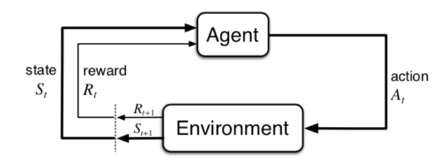
The agent interacts with the environment over time and generate a sequence or trajectory:

\[\tau = \{ S_0, A_0, R_1, S_1, A_1, R_2, S_2, A_2, R_3, \cdots \}\]

Markov Property

A state $S_t$ is Markov if and only if

\[\mathbb{P}\left[S_{t+1} | S_{t}\right]=\mathbb{P}\left[S_{t+1} | S_{1}, \ldots, S_{t}\right]\]

that means the state is a sufficient statistic of the future. For a Markov state $s$ and successor state $s^{\prime}$, the state transition probability is defined by

\[\mathcal{P}_{s s^{\prime}}=\mathbb{P}\left[S_{t+1}=s^{\prime} | S_{t}=s\right]\]

and we have state transition matrix $ \mathcal{P} $ as:

\[\mathcal{P} = \left[\begin{matrix} \mathcal{P}_{11} & \cdots & \mathcal{P}_{1n} \\ \vdots & & \vdots \\ \mathcal{P}_{n1} & \cdots & \mathcal{P}_{nn} \end{matrix}\right]\]

where each row of the matrix sums to $1$.

Markov Process

A Markov Process (or Markov Chain) is a tuple $\langle\mathcal{S}, \mathcal{P}\rangle$ ,

• $\mathcal{S}$ is a (finite) set of states
• $\mathcal{P}$ is a state transition probability matrix

For example, below defines a Markov Chain of student activities in a day:

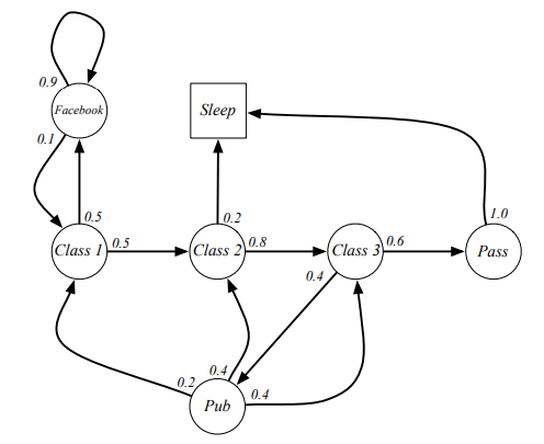
where we can sample episodes with different states.

Markov Reward Process

A Markov Process (or Markov Chain) is a tuple $\langle\mathcal{S}, \mathcal{P}, \mathcal{R}, \gamma \rangle$ ,

• $\mathcal{S}$ is a (finite) set of states
• $\mathcal{P}$ is a state transition probability matrix

\[\mathcal{P}_{s s^{\prime}}=\mathbb{P}\left[S_{t+1}=s^{\prime} | S_{t}=s\right]\]

• $\mathcal{R}$ is a reward function, \(\mathcal{R}_{s}=\mathbb{E}\left[R_{t+1} \mid S_{t}=s \right]\)
• $\gamma$ is a discount factor, $ \gamma \in[0,1]$ , which is used to define the total discounted reward from time-step $t$

\[G_{t}=R_{t+1}+\gamma R_{t+2}+\ldots=\sum_{k=0}^{\infty} \gamma^{k} R_{t+k+1}\]

For example, below defines a Markov Reward Process of student activities in a day:

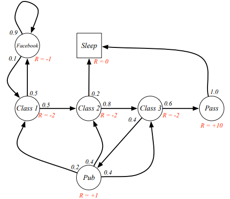
The discount factor is used to avoid infinite returns in infinite horizon, which will reduce the uncertainty about the future may not be fully represented.

Markov Decision Process

A Markov decision process is a Markov reward process with decisions, which can be defined by a tuple $\langle\mathcal{S}, \mathcal{A}, \mathcal{P}, \mathcal{R}, \gamma \rangle$

• $\mathcal{S}$ is a (finite) set of states
• $\mathcal{A}$ is a finite set of actions
• $\mathcal{P}$ is a state transition probability matrix

\[\mathcal{P}_{s s^{\prime}}^{a}=\mathbb{P}\left[S_{t+1}=s^{\prime} \mid S_{t}=s, A_{t}=a\right]\]

• $\mathcal{R}$ is a reward function, \(\mathcal{R}_{s}^{a}=\mathbb{E}\left[R_{t+1} \mid S_{t}=s, A_t = a \right]\)
• $\gamma$ is a discount factor, $ \gamma \in[0,1] $

For example, below defines a Markov Decision Process of student activities in a day:

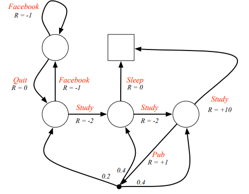
Another reason of using discounted factor is the decision $A_t$ typically has discounted effect on the future rewards $R_{t+k}$, which supposed to be effected by $A_{t+k-1}$.

Ergodic MDP

An ergodic Markov process has a limiting stationary distribution, which is a vector $d(\mathcal{S})$ about state distribution , such that \(d(\mathcal{S}) = d(\mathcal{S}) \cdot \mathcal{P}\)

or

\[d(s)=\sum_{s^{\prime} \in \mathcal{S}} d\left(s^{\prime}\right) \mathcal{P}_{s^{\prime} s}\]

It means over the long run, no matter what the starting state was, the proportion of time the chain spends in state $s$ is approximately $d(s)$, where $\sum_{s \in \mathcal{S} } d(s)$ = 1.0 .

An MDP is ergodic if the Markov chain induced by any policy is ergodic. For any policy $\pi$ , an ergodic MDP has an average reward per time-step $\rho^{\pi}$ that is independent of start state

\[\rho^{\pi}=\lim _{T \rightarrow \infty} \frac{1}{T} \mathbb{E}\left[\sum_{t=1}^{T} R_{t}\right]\]

Goal of an Agent

The goal of an agent is to maximize the expected value of the cumulative sum of a reward, which an agent receives in the long run. In general, the agent seeks to maximize the expected return, which is denoted by $\mathbb{E}[G_t]$. In episodic tasks, which means there exists finite steps of agent-environment interaction, the return can be generally expressed as

\(G_1 = R_{1} + R_{2} + \cdots + R_{T} = R_{1} + G_{2}\) However, if the agent continually interacts with the environment without limit, which is called continuing tasks, we need another form of return

\[G_1 = R_{1} + \gamma R_{2} + \gamma^2 R_{3} + \cdots = \sum_{t=0}^{\infty} \gamma^{t} R_{t+1} = R_{1} + \gamma \cdot G_{2}\]

The intermediate reward usually is designed by human, and keep in mind that, the reward signal is your way of communicating to the robot or agent what you want it to achieve, not how you want it achieved. If you want to give prior knowledge about how we want it to achieve, we might impact the initial policy or initial value function.

Bellman Equations

State-value Function: the value of a state $s$ under policy $\pi$ is defined as

\[v_{\pi}(s)=\mathbb{E}_{\pi}\left[G_{t} | S_{t}=s\right]=\mathbb{E}_{\pi}\left[\sum_{k=0}^{\infty} \gamma^{k} R_{t+k+1} | S_{t}=s\right] \quad \forall s \in S\]

which denotes by the expected return of state $s$ under policy $\pi$ . If $s$ is a terminated state, then $v_{\pi}(s) = 0$.

Action-value Function: the value of a state-action pair under policy $\pi$ is defined as

\[q_{\pi}(s, a) = \mathbb{E}_{\pi}[G_{t} | S_t = s, A_t = a] = \mathbb{E}_{\pi} [\sum_{k=0}^{\infty} \gamma^k R_{t+k+1} |S_t =s , A_t=a] \ \ \ \ \forall s \in \mathcal{S},a \in \mathcal{A}\]

which denotes by the expected return of state $s$ with action $a$ committed under policy $\pi$.

Advantage Function: the difference between action-value and state value,

\[A_{\pi}(s, a) = q_{\pi}(s, a) - v_{\pi}(s, a)\]

which represents how good is a specific action compared with average performance of other actions.

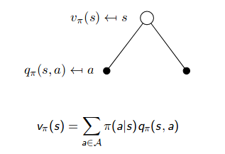
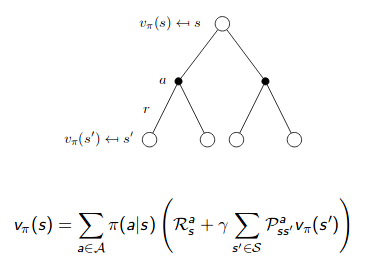
Bellman Expectation Equation for $v_{\pi}(s)$

\[\begin{aligned} v_{\pi}(s) &=\mathbb{E}_{\pi}\left[G_{t} | S_{t}=s\right]=\mathbb{E}_{\pi}\left[\sum_{k=0}^{\infty} \gamma^{k} R_{t+k+1} | S_{t}=s\right] \quad \forall s \in S \\ &=\mathbb{E}_{\pi}\left[R_{t+1}+\gamma G_{t+1} | S_{t}=s\right] \\ &=\mathbb{E}_{\pi}\left[R_{t+1}+\gamma v_{\pi}\left(S_{t+1}\right) | S_{t}=s\right] \\ &=\sum_{a} \pi(a | s) \sum_{r, s^{\prime}} p\left(s^{\prime}, r | s, a\right)\left[r + \gamma v_{\pi}\left(s^{\prime}\right)\right] \\ &=\sum_{a} \pi(a | s) \cdot q_{\pi}(s, a) \end{aligned}\]

The inner summation is to compute the expected return of state $s$ with a specific action $a$. The outer summation is to compute the expected return of state $s$ with all possible actions. We can use two backup diagrams to represent it:

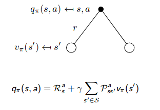
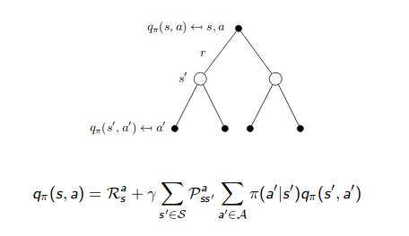
Bellman Expectation Equation for $ q_{\pi}(s, a)$

\[\begin{aligned} q_{\pi}(s, a) &=\mathbb{E}_{\pi}\left[G_{t} | S_{t}=s, A_{t}=a\right]=\mathbb{E}_{\pi}\left[\sum_{k=0}^{\infty} \gamma^{k} R_{t+k+1} | S_{t}=s, A_{t}=a\right] \quad \forall s \in \mathcal{S}, a \in \mathcal{A} \\ &=\mathbb{E}_{\pi}\left[R_{t+1}+\gamma v_{\pi}\left(S_{t+1}\right) | S_{t}=s, A_{t}=a\right] \\ &=\sum_{r, s^{\prime}} p\left(s^{\prime}, r | s, a\right)\left[r+ \gamma v_{\pi}\left(s^{\prime}\right)\right] \end{aligned}\]

We can also use two backup diagrams to represent it:

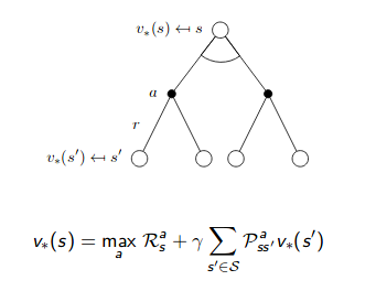
Bellman Optimality Equation for $v_{\pi}(s)$

If we have already known the optimal policy where

\[\begin{aligned} v_{*}(s) &=\max _{\pi} v_{\pi}(s) \\ q_{*}(s, a) &=\max _{\pi} q_{\pi}(s, a) \end{aligned}\]

we can get that

\[v_{*}(s)=\max _{a} q_{*}(s, a) \quad \forall s \in \mathcal{S}\]

that means the value of a state under an optimal policy must equal the expected return for the best action from that state. If it is deterministic action, all actions except the optimal action have $q_{\star}(s, a) = 0$ , since $\pi^{\star}(a \mid s) = 1.0$ for optimal action $a$ .

\[\begin{align} v_{*}(s) &= \max_{a} q_{*}(s,a) \\ &= \max_{a} \mathbb{E}_{\pi^*}[G_t | S_t = s, A_t = a] \\ &= \max_{a} \mathbb{E}_{\pi^*}[R_{t+1} + \gamma G_{t+1} | S_t = s, A_t = a] \\ &= \max_{a} \mathbb{E}_{\pi^*}[R_{t+1} + \gamma v_{*}(S_{t+1}) | S_t = s, A_t = a] \\ &= \max_{a}\sum_{r,s'} p(s', r |s, a) [r + \gamma v_{\pi^{*}}(s')] \\ &= \pi^{*}(a|s) \sum_{r,s'} p(s', r |s, a) [r + \gamma v_{\pi^{*}}(s')] \end{align}\]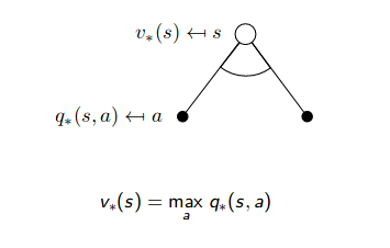

Bellman Optimality Equation for $q_{\pi}(s, a)$

\[\begin{align} q_{*}(s, a) &= \mathbb{E}_{\pi^*}[G_{t} | S_t = s, A_t = a] \\ &= \mathbb{E}_{\pi^*}[R_{t} + \gamma G_{t+1} | S_t = s, A_t = a] \\ &= \mathbb{E}_{\pi^*}[R_{t+1} + \gamma v_{*}(S_{t+1}) | S_t = s, A_t = a] \\ &= \mathbb{E}_{\pi^*}[R_{t+1} + \gamma \max_{a'} q_{*}(S_{t+1}, a') | S_t = s, A_t = a] \\ &= \sum_{r,s'} p(s', r |s, a) [r + \gamma \max_{a'} q_{\pi^{*}}(s', a')] \end{align}\]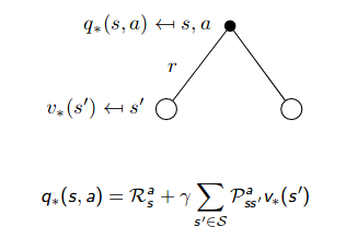

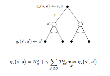The way to check if it is an optimal policy is simply to evaluate if the Bellman optimality equation holds.

Generalized Policy Iteration

The generalized policy iteration refers to the general idea of interleaving policy evaluation and policy improvement, where the policy is always being improved w.r.t the current value function and the current value function is always being driven toward a better value function for the policy.

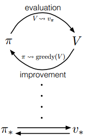
Both processes stabilize only when a policy has been found that is greedy w.r.t its own evaluation function, which implies that the Bellman optimality equation holds. Almost all reinforcement learning methods are well described as GPI.

Policy Evaluation

Starting with a random guess of value function $v_0$, we utilize the Bellman expectation equation as update rule to iteratively update the value function to make more accurate prediction on state-value and action-value under current fixed policy:

\[\begin{aligned} v_{k+1}(s) & \doteq \mathbb{E}_{\pi}\left[R_{t+1}+\gamma v_{k}\left(S_{t+1}\right) | S_{t}=s\right] \\ &=\sum_{a} \pi(a | s) \sum_{s^{\prime}, r} p\left(s^{\prime}, r | s, a\right)\left[r+\gamma v_{k}\left(s^{\prime}\right)\right] \end{aligned}\]

Notice that, the exact policy evaluation requires known MDP, which can be implemented by dynamic programming. If we have unknown MDP, then we have to estimate the policy evaluation according to model-free prediction.

Policy Improvement

Once we complete the policy evaluation and get a fixed most accurate value function for current policy, we can try to improve the policy greedily base on one simple update rule that:

\[q_{\pi} (s, \pi^{\prime}(s)) \geq v_{\pi}(s) \ \ \ \ \ \ \forall s \in \mathcal{S}\]

where $\pi’(s) = \arg\max_{a} q_{\pi} (s, a)$ . We can tweak the policy by choosing the best action for each state based on derived value function for current policy $ \pi$, and we can view it as an optimization of action-value function w.r.t action space under current fixed policy $\pi$. Then the policy $ \pi’$ must be as good as or better than $ \pi$ , under our current value function, that is

\[v_{\pi'}(s) \geq v_{\pi}(s)\]

Since the policy improvement is based on the policy evaluation on current policy which requires model dynamic and finite MDP for exact evaluation, we only can approximately improve the policy based on approximated policy evaluation with model-free methods if we do not know them. The question here is how can we guarantee to improve the policy based on approximated policy evaluation ?

Planning by Dynamic Programming for Known MDP

Policy Iteration

Policy iteration is an algorithm or a procedure of alternatively completing policy evaluation and policy improvement, and eventually makes Bellman optimality equation hold.

\[\pi_{0} \xrightarrow{Eval.} v_{\pi_{0}} \xrightarrow{Impro.} \pi_{1} \xrightarrow{Eval.} v_{\pi_{1}} \xrightarrow{Impro.} \cdots \xrightarrow{Eval.} \pi_{*} \xrightarrow{Eval.} v_{\pi_{*}}\]

For completing the policy evaluation, it may require several sweeps over all states. Making the policy greedy with respect to the value function typically makes the value function incorrect for the changed policy, and making the value function consistent with the policy typically causes that policy no longer to be greedy.

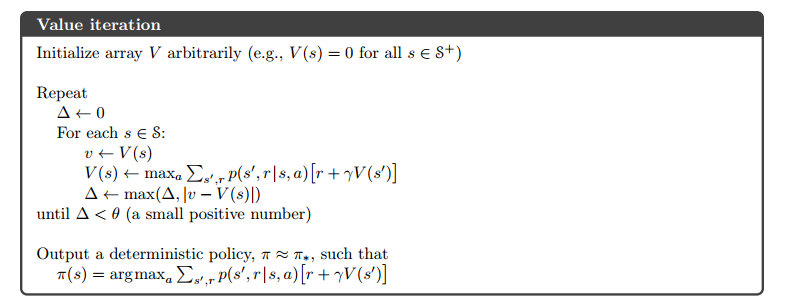
Value Iteration

Value iteration is a revised algorithm of policy iteration, which avoid multiple sweeps on all states during policy evaluation. Value iteration improves the policy as soon as it gets an evaluation of current state, which combines the policy improvement and truncated policy evaluation steps into one simple update operation:

\[\begin{aligned} v_{k+1}(s) & \doteq \max _{a} \mathbb{E}\left[R_{t+1}+\gamma v_{k}\left(S_{t+1}\right) | S_{t}=s, A_{t}=a\right] \\ &=\max _{a} \sum_{s^{\prime}, r} p\left(s^{\prime}, r | s, a\right)\left[r+\gamma v_{k}\left(s^{\prime}\right)\right] \end{aligned}\]

As we can see in the operation above, we do not observe the exact policy improvement step, however we can see that the value function is updated to evaluate the improved policy. This operation also can be viewed as an update rule derived from the Bellman optimality equation.

Model Free Approach

We can utilize the state-value function with dynamic programming to find the optimal policy if we know the state transition probability. However, it is often that we do not have the known MDP, and we have to seek the help of model-free methods, which leverage the action-value function instead. There are two major classes of model-free methods: Monte-Carlo method for episodic tasks and temporal-difference method for continuous tasks. Both MC and TD methods can estimate the state-value function $V_{\pi}(s) $ without a model, however, state-value alone is not sufficient to determine a policy. Therefore, we only study the MC and TD methods for policy evaluation and improvement with action-value function $Q_{\pi}(s, a)$ here. Once we find the optimal action-value function $Q_{*}(s, a)$, we can recover an optimal policy by

\[\pi_{*}(s)=\arg \max _{a} Q_{*}(s, a)\]

One drawback of model-free methods is we need many samples of trajectories. One question here is how many samples are sufficient ? Can we do smart sampling ?

We refer to TD and Monte Carlo updates as sample updates because they involve looking ahead to a sample successor state (or state-action pair), using the value of the successor and the reward along the way to compute a backed-up value, and then updating the value of the original state (or state-action pair) accordingly. Sample updates differ from the expected updates of DP methods in that they are based on a single sample successor rather than on a complete distribution of all possible successors.

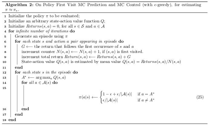
Monte-Carlo Prediction and Control

MC methods are used in episodic tasks that we can sample the full episodes.

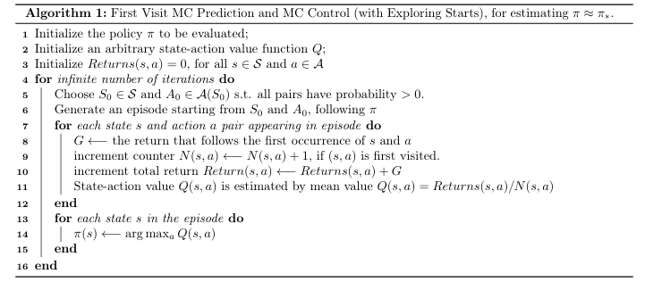
By the law of large numbers, $ Q_{\star} (s,a) \longleftarrow Q_{\pi}(s, a)$ as $N(s,a) \longrightarrow \infty$, and thus $\pi \approx \pi_*$. (Step 7 - Step 12) is policy evaluation, and (Step 13 - Step 15) is policy improvement, which follows value iteration (also the generalized policy iteration). We use the exploring starts to ensure every pair of state and action has probability $>0$ to be visited.

In the algorithm above, we need to keep track of the counter and returns. However, we cannot remember everything in real life, especially when state space and action space is very large. We can replace the (Step 9 - Step 11) with a running mean update:

\[Q(s, a) = Q(s, a) + \alpha (G - Q(s, a))\]

Because

\[\begin{align} \mu_k &= \frac{1}{k} \sum_{j=1}^{k} x_j \\ &= \frac{1}{k} (x_k + \sum_{j=1}^{k-1} x_j) \\ &= \frac{1}{k} (x_k + (k-1) \mu_{k-1}) \\ &= \mu_{k-1} + \frac{1}{k} (x_k - \mu_{k-1}) \end{align}\]

Therefore, we do not need to keep track of the $Returns(s,a)$ after each episode by setting:

\[\begin{align} N(s,a) &\longleftarrow N(s,a) + 1 \\ Q(s,a) &\longleftarrow Q(s,a) + \frac{1}{N(s,a)} (G - Q(s,a)) \end{align}\]

In addition, we can further avoid tracking the $N(s,a)$ by replacing it with $\alpha$. Thus, we can totally forget about the old episodes.

The reason we use the equation (25) is because it still guarantees policy improvement towards optimum, at the meantime, it ensures the exploration to avoid some states are not visited ever in the sampled episodes.

For any $\epsilon$-greedy $\pi$, the $\epsilon$-greedy policy $\pi^{\prime}$ with respect to $Q_{\pi}$ is an improvement, that is $V_{\pi^{\prime}}(s) \geq V_{\pi}(s)$.

\[\begin{aligned} Q_{\pi}\left(s, \pi^{\prime}(s)\right) &=\sum_{a \in \mathcal{A}} \pi^{\prime}(a | s) Q_{\pi}(s, a) \\ &=\epsilon / m \sum_{a \in \mathcal{A}} Q_{\pi}(s, a)+(1-\epsilon) \max _{a \in \mathcal{A}} Q_{\pi}(s, a) \\ & \geq \epsilon / m \sum_{a \in \mathcal{A}} Q_{\pi}(s, a)+(1-\epsilon) \sum_{a \in \mathcal{A}} \frac{\pi(a | s)-\epsilon / m}{1-\epsilon} Q_{\pi}(s, a) \\ &=\sum_{a \in \mathcal{A}} \pi(a | s) Q_{\pi}(s, a) \\ &=V_{\pi}(s) \end{aligned}\]

After we improve the policy, we also use the improved policy to generate next episode, that is the meaning of on-policy. If the episode is generated by another policy which is different from the policy we are trying to learn, then it is called off-policy. Typically, we leverage importance sampling to help off-policy MC methods, and we will discuss it later in off-policy gradient methods. However, the Q-Learning is a special off-policy method that does not require important sampling.

For every-visit Monte-Carlo policy evaluation, it is same as the first-visit MC prediction, except increment the counter $N(s,a)$ and $Returns(s,a)$ when every visit of state-action pair (s,a).

Temporal-Difference Prediction and Control

In many scenarios, we need to handle the continuing tasks that do not have a terminated step. We have to learn from the incomplete episodes by bootstrapping, which means to update a guess of action value function towards a guess of $G$.

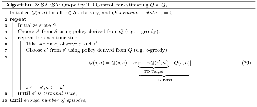
We can see that the main difference between general update in MC methods and in SARSA, is

• MC methods wait until the return (final outcome) $G$ following the visit of $(s,a)$ is known, then use that return as a target for $Q(s,a)$. TD can learn without the final outcome.
• Whereas Monte Carlo methods must wait until the end of the episode to determine the increment to $Q(s,a)$ (only then is $G$ known). TD methods need to wait only until the next time step. At next step on visit of $(s’,a’)$, they immediately form a target and make a useful update using the observed reward $r$ and the estimate $Q(s’,a’)$. In effect, the target for MC is G, whereas the target for TD(0) is $r + \gamma Q(s’, a’)$ .
• In addition, if we are estimating the $V \approx V_{*}$, the updating rule is similar:

\[V(s) = V(s) + \alpha [r + \gamma V(s') - V(s)]\]

• TD and DP both are bootstrapping, but TD does not need to know the model dynamic.

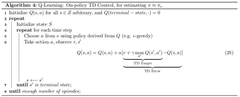
The main difference of SARSA and Q-Learning are:

• SARSA is an on-policy method, and Q-Learning is a off-policy method.
• Q-Learning chooses action at state $s$ following the behavior policy, whereas it updates the Q function assuming we are taking action that maximize $Q(s’,a)$.
• Another way of understanding Q-Learning is by reference to the Bellman optimality equation. The learned action-value function, $Q$, directly approximates the optimal action-value function $Q_*$, independent of the policy being followed.
• Q-Learning learns the optimal policy (by greedy policy) even when actions are selected according to a more exploratory or even random policy.
• If we change the update rule in Q-Learning to following, we get method call expected-SARSA.

\[Q(s,a) = Q(s,a) + \alpha[r + \gamma \sum_{a'} \pi(a'|s') Q(s', a') - Q(s,a)]\]

• Q-Learning can be viewed as Max-SARSA.

Advantages and Disadvantages of MC vs. TD

• TD can learn before knowing the final outcome; MC must wait until end of episode before return is known.
• TD can learn without the final outcome; TD can learn from incomplete sequences; MC can only learn from complete sequences.
• MC has high variance, zero bias; The reason is MC uses the return $G$ as target, which depends on many random actions, transitions, rewards.
  • Good convergence properties (even with function approximation)
  • Not very sensitive to initial value
  • Very simple to understand and use
• TD has low variance, some bias. TD uses the $r + \gamma Q(s’, a’)$ as target, which depends on one random action, transition, reward.
  • Usually more efficient than MC
  • TD(0) converges to $v_{\pi}(s)$ (but not always with function approximation)
  • More sensitive to initial value
• TD exploits Markov property, which is usually more efficient in Markov environments; MC does not exploit Markov property, which is usually more efficient in non-Markov environments.

MC Backup Diagram	TD Backup Diagram	DP Backup Diagram

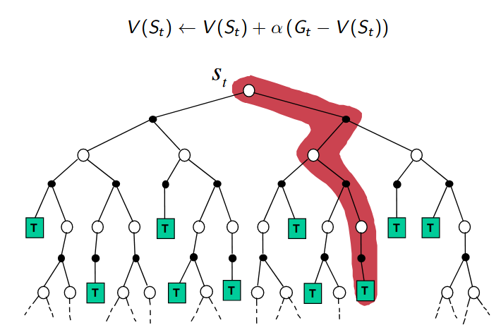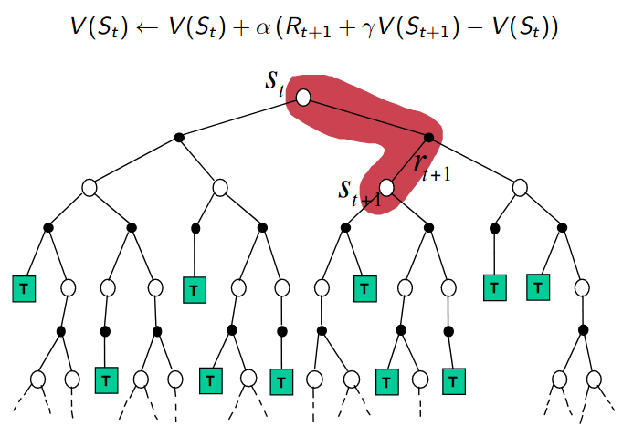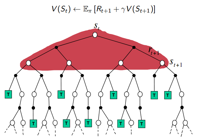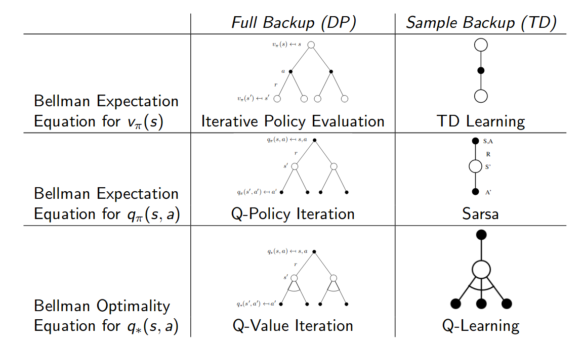
Relationship Between DP and TD

Reference

[1] David Silver’s Lectures

[2] Sutton’s Reinforcement Learning Book