Multi-armed Bandits: Thompson Sampling
Thompson sampling is a well-known multi-armed bandits algorithm for solving exploitation and exploration problem, which is also known as posterior sampling and probability matching. In this post, we will cover Bernoulli bandit problems, sequential recommendation, and reinforcement learning in MDPs with Thompson sampling. Most importantly, we will discuss when, why, and how to apply Thompson sampling.
Bernoulli Bandit Problem with TS
Suppose there is a $K$-arms (actions) bandits, and each action yields either a success (reward $= 1$) or a failure (reward $= 0$). Action \(k \in \{1, \cdots, K \}\) has a hidden probability $\theta_k \in [0, 1]$ that produces a success, which is unknown to the agent, but fixed over time. The objective of the Bernoulli bandit is to learn or estimate the hidden probabilities for all arms by experimentation within $T$ periods, as well as to maximize the cumulative number of successes in $T$ periods.
Beta-Bernoulli Bandit
Each $\theta_{k}$ can be interpreted as an action’s success probability or mean reward. The mean rewards $\theta = (\theta_1, \cdots, \theta_K)$ are unknown, but fixed over time. For instance, an action $x_1$ is applied, and a reward $r_1 \in {0,1} $ is generated with success probability $P(r_1 = 1 \mid x_1, \theta) = \theta_{1}$ .
Now, if we assume an independent beta prior distribution over each $\theta_k$ with hyper-parameters $\alpha = (\alpha_1, \cdots, \alpha_K)$ and $\beta = (\beta_1, \cdots, \beta_K)$, which could be mathematically formalized as:
\[p\left(\theta_{k}\right)=\frac{\Gamma\left(\alpha_{k}+\beta_{k}\right)}{\Gamma\left(\alpha_{k}\right) \Gamma\left(\beta_{k}\right)} \theta_{k}^{\alpha_{k}-1}\left(1-\theta_{k}\right)^{\beta_{k}-1}\]It is very convenient to update each action’s posterior distribution because of the beta-binomial conjugacy:
\[\left(\alpha_{k}, \beta_{k}\right) \leftarrow\left\{\begin{array}{ll} \left(\alpha_{k}, \beta_{k}\right) & \text { if } x_{t} \neq k \\ \left(\alpha_{k}, \beta_{k}\right)+\left(r_{t}, 1-r_{t}\right) & \text { if } x_{t}=k \end{array}\right.\]The parameters $(\alpha_k, \beta_k)$ are sometimes called pseudo- counts, since $\alpha_k$ or $\beta_k$ increases by one with each observed success or failure, respectively. A beta distribution with parameters $(\alpha_k, \beta_k)$ has mean $\alpha_k/(\alpha_k, \beta_k)$, and the distribution becomes more concentrated as $(\alpha_k, \beta_k)$ grows. For example, the figure below
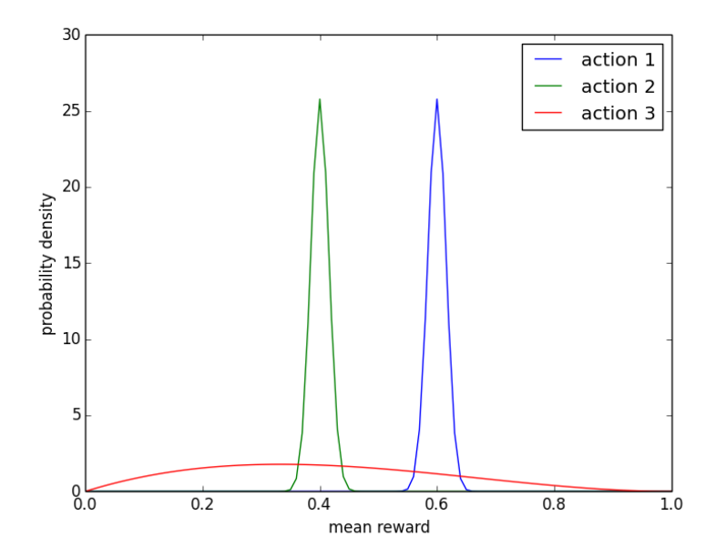 |
|---|
| Figure 1. Probability density functions (Beta distribution) over mean rewards. |
Greedy vs TS
The only difference between greedy policy and Thompson sampling is that the success probability estimate $\hat{\theta}_k$ is randomly sampled from the posterior distribution, which is a beta distribution with parameter $\alpha_k$ and $\beta_k$ , rather than taken to be the expectation $\alpha_k /(\alpha_k + \beta_k)$ .
For example, in figure 1, the greedy algorithm will forgo the potential high reward from action $3$. The worst case is, the greedy algorithm will get stuck on a poor action repeatedly. With $\epsilon$-exploration, equal chances would be assigned to probing action $2$ and $3$, however, action $2$ is extremely unlikely to be optimal.
TS, on the other hand would sample actions $1,2$ and $3$ from the posterior distributions. In the figure 1, you can see that action $3$ has some chance to have mean reward greater than action $1$. Also, the action $2$ has extremely low chance to be selected.
General Thompson Sampling
Now, let’s generalize the Bernoulli bandit problem into a more general setting, where
- the agent could select action $x_{t}$ from a finite or an infinite set $\mathcal{X}$
- after applying action $x_t$ , the agent observes an outcome $y_{t}$, which is generated by the system according to a conditional probability $q_{\theta}(\cdot \mid x_t)$
- the agent receives a reward $r_t = r(y_t)$, where $r$ is a known reward function
- a prior distribution $p$ over the hidden value of $\theta$
We can formulate the expected reward as
\[\mathbb{E}_{q_{\hat{\theta}}}\left[r\left(y_{t}\right) | x_{t}=x\right]=\sum_{o} q_{\hat{\theta}}(o | x) r(o)\]and the conditional distribution as
\[\mathbb{P}_{p, q}\left(\theta=u | x_{t}, y_{t}\right)=\frac{p(u) q_{u}\left(y_{t} | x_{t}\right)}{\sum_{v} p(v) q_{v}\left(y_{t} | x_{t}\right)}\]Specifically, in Bernoulli bandit,
- $\mathcal{X} = {1,\cdots, K}$
- only rewards are observed, that is $y_t = r_t \in {0, 1}$
- observations and rewards are modeled by conditional probabilities $q_{\theta}(1 \mid k) = \theta_k$ and $q_{\theta}(0 \mid k) = 1 - \theta_{k}$
- the prior distribution of $\theta$ is beta distribution with vectors $\alpha$ and $\beta$
Greedy vs TS
The greedy algorithm and Thompson sampling differ in the way they generate model parameters $\hat{\theta}$ , which effects the observations and rewards.
The greedy algorithm estimate $\hat{\theta}$ to be the expectation of $\theta$ with respect to the distribution $p$ at each time stamp, while TS draws a random sample from $p$.
Example: Online Shortest Path
An agent commutes from home to work every morning. She would like to commute along the path that requires the least average travel time, but she is uncertain of the travel time along different routes. How can she learn efficiently and minimize the total travel time over a large number of trips ?
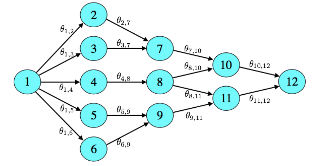 |
|---|
| Figure 2. Shortest Path Problem |
For example, the figure above, it takes $\theta_e$ traveling time on average along an edge $e$ . If there parameters were known, the agent would select (an action) a path $(e_1, \cdots, e_n$), consisting of a sequence of adjacent edges connecting vertices $1$ and $N$, such that the expected total time $\theta_{e_1} + \cdots + \theta_{e_n}$ is minimized. However, the agent does not know the parameters and only could experiment to learn them. In day $t$ , the agent selects a path $x_t = (e_1, \cdots, e_n)$ and observe the realized total traveling time $c_t = \sum_{e\in x_t} y_{t, e}$ , where $y_{t,e}$ is the realized traveling time for each edge along the path $x_t$ . By exploring intelligently, she hopes to minimize cumulative travel time $\sum_{t=1}^{T} c_t $ over a large number of days $T$.
Log-Normal Distribution
The log-normal distribution is the probability distribution of a random variable whose logarithm follows a normal distribution. It models phenomena whose relative growth rate is independent of size, which is true of most natural phenomena including the size of tissue and blood pressure, income distribution, and even the length of chess games.
Let Z be a standard normal variable, which means the probability distribution of Z is normal centered at 0 and with variance 1. Then a log-normal distribution is defined as the probability distribution of a random variable
\[X = e^{\mu+\sigma Z},\]where $\mu$ and $\sigma$ are the mean and standard deviation of the logarithm of X, respectively. The term “log-normal” comes from the result of taking the logarithm of both sides:
\[\log X = \mu +\sigma Z\]Therefore, the definition of log-normal distribution is \(f_X(x) = \frac{1}{x}\frac{1}{\sigma \sqrt{2\pi}}e^{-\dfrac{(\ln x-\mu)^2}{2\sigma^2}},\)
The mean and variance of $X$ could be derived as
\[\mathbb{E}[X] = \exp(\mu + \frac{\sigma^2}{2})\] \[Var[X] = (\exp(\sigma^2) - 1) \exp(2\mu + \sigma^2) = (\exp(\sigma^2) - 1)\cdot \mathbb{E}^2[X]\]Formulation
Now, consider that a travel time $y_{t,e}$ is independently sampled from a distribution with mean $\theta_e$ , and we could set the negative cost as reward, that is:
\[r_t = -\sum_{e\in x_t} y_{t, e}\]Suppose the agent is uncertain about average travel time $\theta_{e}$, and she assumes a prior for which each $\theta_e$ is independent and log-Gaussian distributed[3] with mean $\mu_e$ and variance $\sigma_e^2$. That is
\[\ln(\theta_e) \sim \mathcal{N}(\mu_e, \sigma_e^2)\]We can derive the expectation of $\theta_e$ (log-normal distributed) is
\[\mathbb{E}[\theta_e] = \exp(\mu_e + \frac{\sigma_e^2}{2})\]Further, we assumed that an observed travel time $y_{t,e}$ is independently sampled from a distribution with mean $\theta_e$, that is
\[\mathbb{E}[y_{t,e}\mid \theta_e] = \theta_e\]we could also make $y_{t,e} \mid \theta$ is independently log-Gaussian distribution with mean $\ln(\theta_e) - \frac{\tilde{\sigma}^2}{2}$ and variance $\tilde{\sigma}^2$, therefore, obtain
\[\mathbb{E}[y_{t,e}\mid \theta] = \exp(\ln(\theta_e)- \frac{\tilde{\sigma}^2}{2} + \frac{\tilde{\sigma}^2}{2}) = \theta_e\]For every observation $y_{t,e}$ , we could update the distribution of $\theta_e$ by updating the mean and variance of $\log(\theta_e)$ :
\[\mu_{e}\leftarrow \frac{\frac{1}{\sigma_{e}^{2}} \mu_{e}+\frac{1}{\tilde{\sigma}^{2}}\left(\ln \left(y_{t, e}\right)+\frac{\tilde{\sigma}^{2}}{2}\right)}{\frac{1}{\sigma_{e}^{2}}+\frac{1}{\tilde{\sigma}^{2}}}\] \[\sigma_{e}^{2} \leftarrow \frac{1}{\frac{1}{\sigma_{e}^{2}}+\frac{1}{\tilde{\sigma}^{2}}}\]Reference
[1] Russo, Daniel J., et al. “A tutorial on thompson sampling.” Foundations and Trends® in Machine Learning 11.1 (2018): 1-96.
[2] Chapelle, Olivier, and Lihong Li. “An empirical evaluation of thompson sampling.” Advances in neural information processing systems. 2011.
[3] https://brilliant.org/wiki/log-normal-distribution/
[4]https://en.wikipedia.org/wiki/Log-normal_distribution