Gibbs Sampling with Data Augmentation for Normal Ogive Item Response Theory
[Updated on 05-28-2020] This is a quick note on data augmentation strategy which introduces hidden variables for a handy Gibbs sampling. Two examples are shown for illustration: two-component Gaussian mixture model and Bayesian normal ogive IRT model.
- Data Augmentation for Auxiliary Variables
- Example 1: Two-Component Gaussian Mixture
- Example 2: 2PNO-IRT
- Reference
Data Augmentation for Auxiliary Variables
The idea of data augmentation is to introduce variable $Z$ that depends on the distribution of the existing variables in such as way that the resulting conditional distributions, with $Z$ included, are easier to sample from.
Variable $Z$ could be viewed as latent or hidden variables, which are introduced for the purpose of simplifying or improving the sampler. Suppose we want to sample from $p(x, y)$ with Gibbs sampling, then we need to iteratively sample from $p(x \mid y)$ and $p(y\mid x)$ , which could be very complicated. Therefore, we could choose introduce the hidden variable $Z$ and $p(z\mid x, y)$ such that $p(x\mid y, z)$ , $p(y\mid x, z)$ and $p(z\mid x, y)$ are easy to sample from. In the next step, we could sample all three variables with Gibbs sampling, and throw aways all samples of $Z$ and keep samples (X, Y) from $p(x, y)$.
Example 1: Two-Component Gaussian Mixture
Given a dataset on heights of U.S. 300 women and 400 U.S. men, but we don’t know which data points are from women and which are from men. However, we could have the combined distribution looks like below:
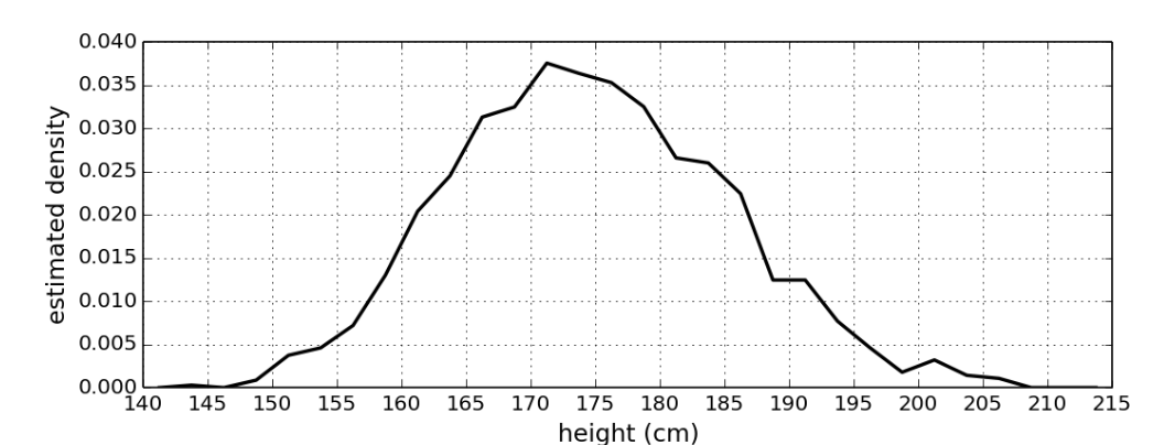 |
|---|
| Heights of women and men, combined. |
This is a two-component mixture of Gaussian, and there should have a unique set of mixture parameters corresponding to any such distribution. Let’s assume that both mixture components have the same fixed and known precision, say $\lambda$. Then, we could formulate the two-component Gaussian mixture model as:
\[\begin{equation} X_1, \cdots, X_n \mid \mu, \pi \sim F(\mu, \pi) \\ \end{equation}\]where $\mu$ denotes the mean of two components, which has a normal distributed prior:
\[\mu := (\mu_0, \mu_1) \sim \mathcal{N}(\nu, \rho^{-1})\]and $\pi$ is the probability for being in the first component and has beta prior:
\[\pi \sim Beta(\alpha, \beta)\]and $F(\mu, \pi)$ is the distribution with p.d.f:
\[f(x \mid \mu, \pi) = (1-\pi) \mathcal{N}(x \mid \mu_0, \lambda^{-1}) + \pi \mathcal{N}(x \mid \mu_1, \lambda^{-1})\]Hence, we have the likelihood
\[\begin{align} p(x_1, \cdots, x_n \mid \mu, \pi) &= \prod_{i=1}^{n} f(x_i \mid \mu, \pi) \\ &= \prod_{i=1}^{n} \left[ (1-\pi) \mathcal{N}(x_i \mid \mu_0, \lambda^{-1}) + \pi \mathcal{N}(x_i \mid \mu_1, \lambda^{-1}) \right] \end{align}\]which is not conjugate with either prior of $\mu$ and prior of $\pi$. Therefore, the posterior distribution cannot be sampled directly.
Solution: Latent Allocation Variables
We could define an equivalent model that includes latent “allocation” variables $Z_1, \cdots, Z_n$ , each of which indicates whether subject $i$ is from female or male.
\[\begin{align} X_i &\sim \mathcal{N}(\mu_{Z_i}, \lambda^{-1}) \ \ \forall i = 1, \cdots, n \\ Z_1, \cdots, Z_n &\sim Bernoulli(\pi) \\ \mu = (\mu_{0}, \mu_{1}) &\sim \mathcal{N}(\nu, \rho^{-1}) \\ \pi &\sim Beta(\alpha, \beta) \end{align}\]and the p.d.f is same as before
\[\begin{align} p(x_i \mid \mu, \pi) &= p(x\mid Z_i=0, \mu, \pi) p(Z_i=0 \mid \mu, \pi) + p(x \mid Z_i=1, \mu, \pi)p(Z_i=1\mid \mu, \pi ) \\ &= \mathcal{N}(x_i \mid \mu_0, \lambda^{-1})(1-\pi) + \mathcal{N}(x_i \mid \mu_1, \lambda^{-1})\cdot \pi \\ &= f(x_i\mid \mu, \pi) \end{align}\]Fully Conditionals
The posterior of parameter $\pi$ is a beta distribution:
\(\begin{align} p(\pi | \mu, z, x)=p(\pi | z)=\operatorname{Beta}\left(\pi | a+n_{1}, b+n_{0}\right) \end{align}\) where $n_0$ and $n_1$ are number of 0s and 1s in ${z_1, \cdot, z_n}$, respectively.
The posterior of $\mu$ is a normal distribution:
\[\begin{align} \mu_0 \mid \mu_1, x, z, \pi &\sim \mathcal{N}(M_0, \Lambda_0^{-1}) \\ \mu_1 \mid \mu_0, x, z, \pi &\sim \mathcal{N}(M_1, \Lambda_1^{-1}) \end{align}\]where for $k \in {0, 1}$,
\[\begin{align} n_{k} &=\sum_{i=1}^{n} \mathbb{1}\left(z_{i}=k\right) \\ M_{k} &=\frac{\rho m+\lambda \sum_{i: z_{i}=k} x_{i}}{\rho+n_{k} \lambda} = \Lambda_k^{-1} (\rho m+\lambda \sum_{i: z_{i}=k} x_{i})\\ \Lambda_{k} &=\rho+n_{k} \lambda \end{align}\]The posterior of all introduced latent allocated variables $Z_1, \cdots, Z_n$ is
\[\begin{align} p(z | \mu, \pi, x) & \propto p(x, z, \pi, \mu) \propto p(x | z, \mu) p(z | \pi) \\ &=\prod_{i=1}^{n} \mathcal{N}\left(x_{i} | \mu_{z_{i}}, \lambda^{-1}\right) \text {Bernoulli }\left(z_{i} | \pi\right) \\ &=\prod_{i=1}^{n}\left(\pi \mathcal{N}\left(x_{i} | \mu_{1}, \lambda^{-1}\right)\right)^{z_{i}}\left((1-\pi) \mathcal{N}\left(x_{i} | \mu_{0}, \lambda^{-1}\right)\right)^{1-z_{i}} \\ &=\prod_{i=1}^{n} \alpha_{i, 1}^{z_{i}} \alpha_{i, 0}^{1-z_{i}} \\ & \propto \prod_{i=1}^{n} \operatorname{Bernoulli}\left(z_{i} | \alpha_{i, 1} /\left(\alpha_{i, 0}+\alpha_{i, 1}\right)\right) \end{align}\]where
\[\begin{align} \alpha_{i, 0} &=(1-\pi) \mathcal{N}\left(x_{i} | \mu_{0}, \lambda^{-1}\right) \\ \alpha_{i, 1} &=\pi \mathcal{N}\left(x_{i} | \mu_{1}, \lambda^{-1}\right) \end{align}\]Example 2: 2PNO-IRT
The two-parameter normal ogive item response theory model is defined as:
\[p_{ij} = \Phi(a_j \theta_i - d_j)\]where $p_{ij}$ denotes is probability of user $i$ response to item $j$ with value 1, $\theta_i$ is $i^{th}$ user’s ability, $d_j$ is $j^{th}$ item’s difficulty, and $a_j$ measures the ability of the item to discriminate between good and poor users.
Consider a set of responses $\mathbf{y} = { y_{ij} \in {0, 1} }$ for $M$ users and $N$ items, the likelihood could be expressed as
\[\begin{align} p(\mathbf{y} \mid \boldsymbol{\theta}, \boldsymbol{d}, \boldsymbol{a}) &= \prod_{i=1}^{M}\prod_{j=1}^{N} p(y_{ij}\mid \theta_i, d_j, a_j) \\ &= \prod_{i=1}^{M}\prod_{j=1}^{N} p_{ij}^{y_{ij}} \cdot (1-p_{ij})^{1-y_{ij}} \end{align}\]Now, assuming the user abilities $\boldsymbol{\theta}$ is given and
\[\theta_1, \cdots, \theta_M \ \text{is a random sample from}\ \mathcal{N(0, 1)}\]The joint density of the response $\mathbf{y}$ and $\boldsymbol{\theta}$ is given by
\[p(\mathbf{y}, \boldsymbol{\theta} \mid \boldsymbol{d}, \boldsymbol{a}) = \prod_{i=1}^{M} \mathcal{N}(\theta_i; 0,1) \prod_{j=1}^{N} p(y_{ij}\mid \theta_i, d_j, a_j)\]With certain prior distributions on $\boldsymbol{d}$ and $\boldsymbol{a}$ , we could have the posterior density of $(\boldsymbol{\theta}, \boldsymbol{d}, \boldsymbol{a})$ , that is
\[\pi(\boldsymbol{\theta} , \boldsymbol{d}, \boldsymbol{a} \mid \mathbf{y}) \propto p(\mathbf{y} \mid \boldsymbol{\theta} , \boldsymbol{d}, \boldsymbol{a}) \cdot \pi(\boldsymbol{\theta})\cdot \pi(\boldsymbol{d}) \cdot \pi(\boldsymbol{a})\]In this post, we use following prior distributions
\[\begin{align} \theta_i &\sim \mathcal{N}(\mu_{\theta},\sigma^2_{\theta}) \\ d_j &\sim \mathcal{N}(\mu_d, \sigma^2_d) \\ a_j &\sim \mathcal{N}_{(0, \infty)}(\mu_a, \sigma^2_a) \end{align}\]Latent Variables
To implement the Gibbs sampler for the joint posterior distribution above, we first introduce random variables $(Z_{11}, \cdots, Z_{MN})$ where $Z_{ij}$ is distributed normal with mean $\eta_{ij} = a_j\theta_i - d_j$ and standard deviation $1$. Suppose $Y_{ij} = 1$ if $Z_{ij} > 0$ and $Y_{ij} = 0$ otherwise. Now, we are interested in simulating from the joint posterior distribution $(\boldsymbol{Z}, \boldsymbol{\theta}, \boldsymbol{\xi})$ , where $\boldsymbol{\xi}_j = [a_j, d_j]^\top$ :
\[p(\boldsymbol{\theta}, \boldsymbol{\xi}, \mathbf{Z} | \mathbf{y}) \propto f(\mathbf{y} | \mathbf{Z}) p(\mathbf{Z} | \boldsymbol{\theta}, \boldsymbol{\xi}) p(\boldsymbol{\theta}) p(\boldsymbol{\xi})\] \[\begin{align} \pi(\boldsymbol{Z}, \boldsymbol{\theta} , \boldsymbol{\xi} \mid \mathbf{y}) &= C\cdot f(\mathbf{y} | \mathbf{Z}) p(\mathbf{Z} | \boldsymbol{\theta}, \boldsymbol{\xi}) \pi(\boldsymbol{\theta}) \pi(\boldsymbol{\xi}) \\ &= C \cdot \prod_{i=1}^{M}\left\{ \mathcal{N}(\theta_i; \mu_{\theta},\sigma_{\theta}) \cdot \prod_{j=1}^{N} \mathcal{N}(Z_{ij}; \eta_{ij}, 1) \left[ \mathbb{I}(Z_{ij} > 0)\cdot \mathbb{I}(y_{ij}=1)) \\ + \mathbb{I}(Z_{ij} \leq 0)\cdot \mathbb{I}(y_{ij}=0))\right] \right\} \prod_{j=1}^{N}\mathcal{N}(\mu_d, \sigma_d^2) \cdot \mathcal{N}(\mu_a, \sigma_a^2)\cdot \mathbb{I}(a_j > 0) \end{align}\]where $\mathbb{I}(\cdot)$ is the indicator function.
The Gibbs sampling involves 3 of the sampling processing, namely, a sampling of the augmented $Z$ parameters, a sampling of person trait $\theta_{i}$ , and a sampling of the item parameter $\boldsymbol{\xi}_j$ .
The posterior of parameter $\boldsymbol{Z}$ is
\[\pi(Z_{ij} \mid \cdot) \propto \mathcal{N}(Z_{ij}; \eta_{ij}, 1) \left[ \mathbb{I}(Z_{ij} > 0)\cdot \mathbb{I}(y_{ij}=1)) + \mathbb{I}(Z_{ij} \leq 0)\cdot \mathbb{I}(y_{ij}=0))\right]\]and we sample it from
\[Z_{i j} | \bullet \sim\left\{\begin{array}{ll} N_{(0, \infty)}\left(\eta_{i j}, 1\right), & \text { if } \quad y_{i j}=1 \\ N_{(-\infty, 0)}\left(\eta_{i j}, 1\right), & \text { if } \quad y_{i j}=0 \end{array}\right.\]The posterior of person trait $\theta_i$ is
\[\pi(\theta_i \mid \cdot) \propto \underbrace{\mathcal{N}(\theta_i; \mu_{0}, \sigma_{0}^2)}_{\text{prior}} \cdot \overbrace{ \prod_{j=1}^{N} \mathcal{N}(Z_{ij}; \eta_{ij}, 1)}^{\text{likelihood}}\]where the likelihood can be expressed as
\[\begin{align} &\prod_{j=1}^{N} \mathcal{N}(Z_{ij}; \eta_{ij}, 1) \\ &\propto \left(\sigma^{2}\right)^{-\frac{N}{2}} \exp\left\{-\frac{1}{\sigma^2} \cdot \sum_{j=1}^{N} \frac{(Z_{ij}-a_j\theta_i + d_j)^{2}}{2}\right\} \\ &= \exp\left\{- \sum_{j=1}^{N} \frac{(Z_{ij}-a_j\theta_i + d_j)^{2}}{2}\right\} \\ &= \exp\left\{- \sum_{j=1}^{N} \frac{(Z_{ij} + d_j)^2-2(a_j\theta_i)(Z_{ij}+d_j) +(a_j\theta_i)^{2}}{2}\right\} \\ &= \exp\left\{- \frac{\sum_{j=1}^{N} (Z_{ij} + d_j)^2- 2\theta_i\sum_{j=1}^{N} a_j(Z_{ij}+d_j) + \theta_i^2\sum_{j=1}^{N} a_j^2}{2}\right\} \\ &= \exp\left\{- \sum_{j=1}^{N} a_j^2 \cdot \frac{\frac{\sum_{j=1}^{N}(Z_{ij} + d_j)^2}{\sum_{j=1}^{N} a_j^2}- \frac{2\theta_i\sum_{j=1}^{N} a_j(Z_{ij}+d_j)}{\sum_{j=1}^{N} a_j^2} + \theta_i^2}{2 }\right\}\\ &= \exp\left\{- \sum_{j=1}^{N} a_j^2 \cdot \frac{(\theta- \frac{\sum_{j=1}^{N} a_j(Z_{ij}+d_j)}{\sum_{j=1}^{N} a_j^2})^2}{2 }\right\} \\ &\propto \mathcal{N}\left(\frac{\sum_{j=1}^{N} a_j(Z_{ij}+d_j)}{\sum_{j=1}^{N} a_j^2} , \frac{1}{\sum_{j=1}^{N} a_j^2} \right) \end{align}\]Based on the conjugacy of Gaussian [4], we can obtain the mean $\mu_n$ and variance $\sigma_n^2$ of posterior distribution on Gaussian as:
\[\mu_n = \sigma_n^2 \left( \frac{\mu_0}{\sigma^2_0} + \frac{\sum_{i}^{n}x_i}{\sigma^2} \right)\] \[\sigma_{n}^{2}=\frac{1}{\frac{n}{\sigma^{2}}+\frac{1}{\sigma_{0}^{2}}}\]where $\mu_0$ and $\sigma_0^2$ are mean and variance of prior distribution, and $n$ is the number of data points, $x_i$ is the data point, and $\sigma^2$ is the variance of likelihood. In our case, $x_i$ is the $\theta_i$ with $n=1$. Therefore, we can sample $\theta_i $ from
\[\theta_{i} | \bullet \sim \mathcal{N}\left(\frac{\sum_{j}\left(Z_{i j}+d_{j}\right) a_{j}+\mu_{0} / \sigma_{0}^{2}}{1 / \sigma_{0}^{2}+\sum_{j} a_{j}^{2}}, \frac{1}{1 / \sigma_{0}^{2}+\sum_{j} a_{j}^{2}}\right)\]Lastly, the posterior of item characteristics $\xi_j$ is
\[\pi(\xi_j \mid \cdot) \propto \underbrace{\mathcal{N}(\xi_i; \mu_{\xi}, \Sigma_{\xi})}_{\text{prior}} \cdot \overbrace{ \prod_{i=1}^{M} \mathcal{N}(Z_{ij}; \eta_{ij}, 1)}^{\text{likelihood}}\]where
\[\boldsymbol{\mu}_{\boldsymbol{\xi}} = [\mu_a, \mu_d]^\top\] \[\boldsymbol{\Sigma}_{\boldsymbol{\xi}}=\left[\begin{array}{cc}\sigma_{\alpha}^{2} & 0 \\ 0 & \sigma_{\beta}^{2} \end{array}\right]\]and the likelihood can be expressed
\[\begin{align} &\prod_{i=1}^{M} \mathcal{N}(Z_{ij}; \eta_{ij}, 1) \\ &\propto \left(\sigma^{2}\right)^{-\frac{N}{2}} \exp\left\{-\frac{1}{\sigma^2} \cdot \sum_{i=1}^{M} \frac{(Z_{ij}-a_j\theta_i + d_j)^{2}}{2}\right\} \\ &= \exp\left\{- \frac{\sum_{i=1}^{M}(Z_{ij})^{2} - \sum_{i=1}^{M}2Z_{ij}(a_j\theta_i-d_j) + \sum_{i=1}^{M}(a_j\theta_i -d_j)^2}{2}\right\} \\ &= \exp\left\{- \frac{\|Z_j\|^2_2 - 2Z_j^\top[\boldsymbol{\theta,-\boldsymbol{1}}]\boldsymbol{\xi}_j + \|[\boldsymbol{\theta}, -\boldsymbol{1}]\boldsymbol{\xi}_j\|^2_2}{2}\right\} \\ &= \exp\left\{- \frac{\|Z_j\|^2_2 - 2Z_j^\top\mathbf{x}\boldsymbol{\xi}_j + \|\mathbf{x} \boldsymbol{\xi}_j\|^2_2}{2}\right\} \\ &= \exp\left\{- \frac{Z_j^\top Z_j - 2Z_j^\top\mathbf{x}\boldsymbol{\xi}_j + (\mathbf{x}\boldsymbol{\xi}_j)^\top(\mathbf{x}\boldsymbol{\xi}_j) }{2}\right\} \\ &= \exp\left\{- \frac{Z_j^\top Z_j - 2Z_j^\top\mathbf{x}\boldsymbol{\xi}_j + \boldsymbol{\xi}_j^\top (\mathbf{x}^\top\mathbf{x})\boldsymbol{\xi}_j }{2}\right\} \\ &= \exp\left\{- (\mathbf{x}^\top\mathbf{x})\cdot \frac{Z_j^\top Z_j - 2Z_j^\top\mathbf{x}\boldsymbol{\xi}_j + \boldsymbol{\xi}_j^\top (\mathbf{x}^\top\mathbf{x})\boldsymbol{\xi}_j }{2(\mathbf{x}^\top\mathbf{x})}\right\} \\ &= \exp\left\{- (\mathbf{x}^\top\mathbf{x})\cdot \frac{ \frac{Z_j^\top Z_j}{\mathbf{x}^\top\mathbf{x}} - 2\frac{Z_j^\top\mathbf{x}\boldsymbol{\xi}_j}{\mathbf{x}^\top\mathbf{x}} + \boldsymbol{\xi}_j^\top \boldsymbol{\xi}_j }{2}\right\} \\ &= \exp\left\{- \frac{ (\boldsymbol{\xi}_j - \frac{Z_j}{\mathbf{x}})^\top (\mathbf{x}^\top\mathbf{x}) (\boldsymbol{\xi}_j -\frac{Z_j}{\mathbf{x}}) }{2}\right\} \\ \end{align}\]where $\mathbf{x} = [\boldsymbol{\theta}, \boldsymbol{1}]$ . Therefore, we have mean of likelihood w.r.t $\boldsymbol{\xi}_j$ as $\frac{Z_j}{\mathbf{x}}$ and variance as $(\mathbf{x}^\top\mathbf{x})^{-1}$ .
Based on the conjugacy of Gaussian [4], we can obtain the mean $\mu_n$ and covariance $\Sigma_{n}$ of posterior distribution on Gaussian as:
\[\begin{align} \Sigma_n &= (\Sigma_0^{-1} + n\Sigma^{-1})^{-1} = (\Sigma_{\xi}^{-1} + \mathbf{x}^\top\mathbf{x})^{-1} \\ \mu_n &= \Sigma_n (n \Sigma^{-1} \bar{x} + \Sigma_{0}^{-1}\mu_0) = (\Sigma_{\xi}^{-1} + \mathbf{x}^\top\mathbf{x})^{-1} ( \mathbf{x}^\top\mathbf{x} \cdot \frac{Z_j}{\mathbf{x}}+ \Sigma_{\xi}^{-1} \mu_{\xi}) \end{align}\]where $\mu_0$ and $\Sigma_0$ are mean and covariance of prior distribution, and $M$ is the number of data points, $x_i$ is the data point, and $\Sigma$ is the covariance of likelihood. In our case, $x_i$ is the $\boldsymbol{\xi}_j$ with $n=1$. Therefore, we can sample $\boldsymbol{\xi}_i $ from
\[\boldsymbol{\xi}_j\mid \bullet \sim \mathcal{N}\left((\Sigma_{\xi}^{-1} + \mathbf{x}^\top\mathbf{x})^{-1} ( \mathbf{x}^\top Z_j+ \Sigma_{\xi}^{-1} \mu_{\xi}) , (\Sigma_{\xi}^{-1} + \mathbf{x}^\top\mathbf{x})^{-1} \right) \mathbb{I}(a_j > 0)\]Reference
[1] Gibbs Sampling and Data Augmentation
[2] Albert, James H. “Bayesian estimation of normal ogive item response curves using Gibbs sampling.” Journal of educational statistics 17.3 (1992): 251-269.
[3] Sheng, Yanyan. “Markov chain Monte Carlo estimation of normal ogive IRT models in MATLAB.” Journal of Statistical Software 25.8 (2008): 1-15.
[4] Conjugate Bayesian analysis of the Gaussian distribution - Kevin P. Murphy