Attention Mechanism [1]: Seq2Seq Models
This is the first note on attention mechanism in deep learning. Neural machine translation will be first introduced for more intuitive understanding.
- Sequence to Sequence Model for Machine Translation
- Neural Machine Translation
- Attention Mechanism
- Reference
Sequence to Sequence Model for Machine Translation
Early Machine Translation
Machine learning (MT) is the task of translating a sentence $x$ from one language (the source language) to a sentence $y$ in another language (the target language). The early systems were mostly rule-based. In 1990s and 2010s, the statistical machine translation (SMT) was the main stream of the MT method, which is to learn a probabilist model from data [8]. For example, if we want to find best English sentence $y$ given French sentence $x$ , the objective is to :
\[\arg\max_{y} P(y \mid x) = \arg\max_{y} \underbrace{P(x\mid y) }_{\text{translate model}}\cdot \underbrace{p(y)}_{\text{language model}}\]where the translation model models how words and phrases should be translated (fidelity) from two languages, and language model models how to write good English (fluency) from monolingual data. For example, the n-gram language model $p(y)$ could be viewed as
\[p(y_1, \cdots, y_n) = p(y_1) p(y_2\mid y_1) \cdots p(y_n \mid y_{n-1})\]where $y_i$ denotes the $i^{th}$ word of sentence $y$. Given a large amount of text data, we could easily compute the $p(y_i\mid y_j)$ based on Baye’s rule.
How to learn translation model $P(x\mid y)$ from the parallel corpus ? We could break it down further by considering a latent variable in the model
\[P(x, a \mid y)\]where $a$ is the alignment, i.e. word-level correspondence between French sentence $x$ and English sentence $y$ .
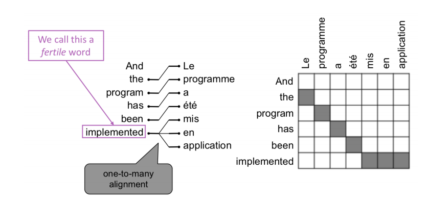
How to represent the $a$ ? We could use matrix $A$ to represent the alignment, where the column corresponds to source sentence and row corresponds to target sentence. We could set $A_{ij} = 1$ if word $i$ in source sentence aligns with the word $j$ in target sentence. So the alignment could be very complex, such that it could be 1 to 1 alignment, 1 to many alignment, many to 1 alignment. or many to many alignment. For example, sometime a single word in one language may require many words to describe.
 |
|---|
| Figure 1. One-to-Many Alignment. |
**How to learn this alignment or $P(x, a\mid y)$ ? **[8] Alignment $a$ are latent variables, which are not explicitly specified in the data. Therefore, given the pair of input and output sentence, we need to use some special learning algorithm (like EM) for learning the parameters of distributions with latent variables.
How to solve the argmax ? The most critical part of this problem is to solve the $argmax_{y} P(x\mid y)\cdot P(y)$ . We could enumerate every possible $y$ and calculate the probability, but it is only feasible if the search space of $y$ is small. Otherwise, we have to resort to a heuristic search algorithm to search for the best translation, discarding hypotheses that are very unlikely. This step of solving the argmax could be understood as decoding for SMT.
SMT was a huge research field, however, the best systems were extremely complex, in where systems had many separately-designed subcomponents.
Neural Machine Translation
The neural machine translation model aims to find a neural network such that output the target sentence directly given the source sentence as input. Briefly, it composes with 2 RNN: encoder RNN and decoder RNN (or LSTM [2]). The encoder RNN encodes the source sentence and provide initial hidden state (or context) for decoder RNN, and then the decoder RNN generates target sentence, conditioned on the provided encoding from encoder RNN. The main different between NMT and SMT is that NMT directly learns the probability $p(y\mid x)$ instead of $p(x\mid y) \cdot p(y)$.
The goal of the encoder and decoder RNN (or LSTM) is to estimate the conditional probability $P(y_1, \cdots, y_{T’} \mid x_1, \cdots, x_T)$ where $(x_1, \cdots, x_T)$ is an input sentence and $(y_1,\cdots , y_{T’})$ is its corresponding output sentence whose length $T’$ may differ from $T$. The neural network computes this conditional probability by first obtaining the fixed dimensional representation $v$ of the input sequence $(x_1, \cdots, x_T)$ given by the last hidden state of the LSTM, and then computing the probability below:
\[p\left(y_{1}, \ldots, y_{T^{\prime}} \mid x_{1}, \ldots, x_{T}\right)=\prod_{t=1}^{T^{\prime}} p\left(y_{t} \mid \color{red}{v}, y_{1}, \ldots, y_{t-1}\right)\]Given a sequence of input $(x_1, \cdots, x_T)$ , a standard RNN computes a sequence of outputs $(y_1,\cdots , y_{T’})$ by iterating the following equation:
\[\begin{array}{l} h_{t}=\operatorname{sigm}\left(W^{\mathrm{hx}} x_{t}+W^{\mathrm{hh}} h_{t-1}\right) \\ y_{t}=W^{\mathrm{yh}} h_{t} \end{array}\]How to train a NMT system ?[1] Given a pair of source sentence and target sentence, we feed the source sentence into the neural network and output a sequence of probabilities of next word (which is represented by a sequence of vectors). In other word, each $P(y_t \mid v, y_1, \cdots, y_{t-1})$ distribution in (3) is represented with a softmax over all words in the vocabulary. The ground truth word is also represented by one-hot encoding, then then we could compute the loss for each word and then average them.
 |
|---|
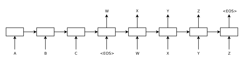
| Figure 2. The model reads an input sentence “ABC” and produces “WXYZ” as the output sentence. The model stops making predictions after outputting the end-of-sentence token [2]. |
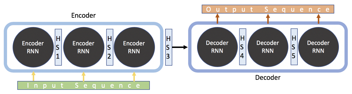
Now, let’s check the detail of this RNN model. By design, RNNs take two inputs: 1. current input at time $t$ and a representation of the previous inputs from time 1 to time $t-1$ . In the end of encoder, the encoder will pass the embedding of input sentence (for example, HS3 in Figure 3) to decoder. The decoder will generate output sentence based on the context (HS3 in figure 3) from input sentence.
 |
|---|
| Figure3. Visualization of Hidden State Processing in NMT [6] |
The most important thing lies in the understanding of decoding, which is essentially to solve the argmax problem (1). There are several ways to decode the input sentence embedding, such as greedy decoding and beam search decoding [8].
One trick suggested in [2] to model the long sentence is to reverse the order of words in the source sentence but not the target sentences in the training and test set. By doing so, the first output of sentence is proximity to the first input of sentence, making it easy for SGD to get a good initial direction to train I think. Intuitively, if the first estimate of word is incorrect, then it is high likely to generate incorrect target sentence, because the next word is generated based on the first word.
This NMT model could be viewed as one seq2seq model [1,2] . There are many NLP tasks can be phrased as seq2seq model. In addition, the seq2seq model is an example of a conditional language model, since the decoder is predicting the next word of the target sentence $y$ , and it is conditioned on the source sentence.
Some disadvantages, limitations, and difficulties of neural machine translation model:
- difficult to interpret and control
- out-of-vocabulary words problem
- domain mismatch between train and test data problem
- maintaining context over longer text problem
- low-resource language pairs problem
- NMT picks up biases in training data
The Bottleneck Problem of Seq2Seq and Attention
The output sentence relies heavily on the context or final representation of input sentence generated by encoder, making it challenging for the model to deal with long sentences. One reason I think is the hidden state representation is typically defined in low dimensional space, and for long sentences the initial context could be easily lost during the encoding process.
To address this issue, [5, 7] introduce “attention” mechanism which allows the model to focus on different parts of the input sequence at every stage of decoding the context of input sentence and generating output sentence. More specifically, on each step of the decoder, it uses direct connection to the encoder to focus on a particular part of the source sentence.
 |
|---|
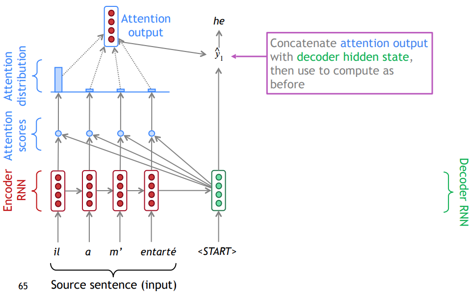
| Figure 4. Visualization of Attention Process. |
After applying encoder, we could obtain $h_1, \cdots, h_T \in \mathbb{R}^h$ $T$hidden states. When generating the first word of target language, the decoder takes the last hidden state of input sentence $h_T$ and empty input (START) to generate first decoder hidden state $s_1 \in \mathbb{R}^{h}$. The next step is to get the attention scores $e^1$:
\[e^1 = [s_1^\top h_1, \cdots, s_1^\top h_T] \in \mathbb{R}^{T}\]Then, we take softmax to get the attention distribution $\alpha^{1}$ for this step:
\[\alpha^1 = softmax(e^1) \in \mathbb{R}^T\]Then, we use $\alpha^1$ to take a weighted sum of the encoder hidden states to get the attention output $\mathbf{a}_1$ :
\[\mathbf{a}_1 = \sum_{i=1}^{T} \alpha_i^1 \mathbf{h}_i \in \mathbb{R}^h\]Finally, we concatenate the attention output $\mathbf{a}_1$ with the decoder hidden state $s_1$ to represent the estimated output of first word in target language: $\hat{y}_1$.
\[\hat{y}_1 = [\mathbf{a}_1; \mathbf{s}_1] \in \mathbb{R}^{2h}\]We continue the similar steps as described above to obtain the whole sentence in target language until we see the output word $\hat{y}_t$ is close to period mark.
Advantages of attention:
-
allows decoder to focus on certain parts of the source and bypass bottleneck
-
helps with vanishing gradient problem, since it provides shortcut to faraway states
-
surprisingly, it provides some interpretability. By inspecting attention distribution, we can see what the decoder was focusing on, and we get soft alignment automatically.
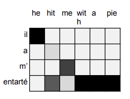
Figure 5. Soft Alignment from Attention Distribution with Explicitly Trained by Alignment System [8]. Thus, attention distribution is often called align scores [7]. The reason I think is the aligned word-pair embeddings lie close to each other in high dimensional space. For example, to train the model to align first word of input and output sentence, it will make the first encoder hidden state close to the first decoder hidden state embedding, so that the attention score is high after dot product.
Attention Mechanism
Definition: Given a set of vector values, and a vector query, attention is a technique to compute a weighted sum of the values, dependent on the query.
For example in NMT (see figure 4), when we apply attention on first stage of decoding, we use all hidden states generated by encoder as a set of vector values and the decoder hidden state as the query vector. The weighted sum is a selective summary of the information contained in the values, where the query determines which values to focus on.
Attention Variants
There are several attention variants [8], and all of them differ on the computing of attention scores $\mathbf{e}\in \mathbb{R}^{T}$. Assume a set of vector values $\mathbf{h}_1, \cdots, \mathbf{h}_T \in \mathbb{R}^{d_1} $ and the query vector $\mathbf{s} \in \mathbb{R}^{d_2}$,
- Basic dot-product attention[7]: $e_i = \mathbf{s}^\top \mathbf{h}_i \in \mathbb{R} $
- this assumes $d_1 = d_2$
- Scaled dot-product attention[13]: $e_i = \frac{\mathbf{s}^\top \mathbf{h}_i}{\sqrt{n}} \in \mathbb{R} $
- where $n = d_1 = d_2$
- Content-based attention [7]: $e_i = cosine(\mathbf{s}, \mathbf{h}_i)$
- Multiplicative attention [7]: $e_{i}=\boldsymbol{s}^{\top} \boldsymbol{W} \boldsymbol{h}_{i} \in \mathbb{R}$
- $\boldsymbol{W}\in \mathbb{R}^{d_2\times d_1}$ is a weight matrix.
- Additive attention [5]: \(e_{i}=\boldsymbol{v}^{\top} \tanh \left(\boldsymbol{W}_{1} \boldsymbol{h}_{i}+\boldsymbol{W}_{2} \boldsymbol{s}\right) \in \mathbb{R}\)
- $\boldsymbol{W}_1 \in \mathbb{R}^{d_3\times d_1}$ , $\boldsymbol{W}_2\in \mathbb{R}^{d_3\times d_2}$, and $\mathbf{v} \in \mathbb{R}^{d_3}$
- $d_3$ (the attention dimensionality) is a hyper-parameter
However, attention always involves 3 steps:
-
computing the attention scores $\mathbf{e}\in \mathbb{R}^{T}$
-
Taking softmax to get attention distribution $\alpha$
\[\alpha=\operatorname{softmax}(\boldsymbol{e}) \in \mathbb{R}^{T}\] -
Using attention distribution to take weighted sum of values:
\[\mathbf{a}=\sum_{i=1}^{T} \alpha_{i} \boldsymbol{h}_{i} \in \mathbb{R}^{d_{1}}\]which is called the context vector. Essentially the context vector consumes 3 pieces of information: encoder hidden states, decoder hidden states, and alignment between source and target.
After obtaining the context vector, there are several ways to obtain the predictive distribution:
- simple concatenation with decoder hidden state $\hat{y} = [\mathbf{a}; \mathbf{s}] $
- concatenation and transformation $\hat{y} = softmax(\boldsymbol{W}_{s}(tanh(\boldsymbol{W}_a[\mathbf{a};\mathbf{s}])))$
In general, attention variants could be categorized into 3 classes:
-
Global attention [7] or soft attention [11]: attention is placed on all source positions, like the way in previous NMT example.
-
Local attention [7]: attention is placed on few source position. Global attention may be expensive and impractical to translate longer sequences such as paragraphs or documents. Refer [7,12] to see ways to select source locations for attention.
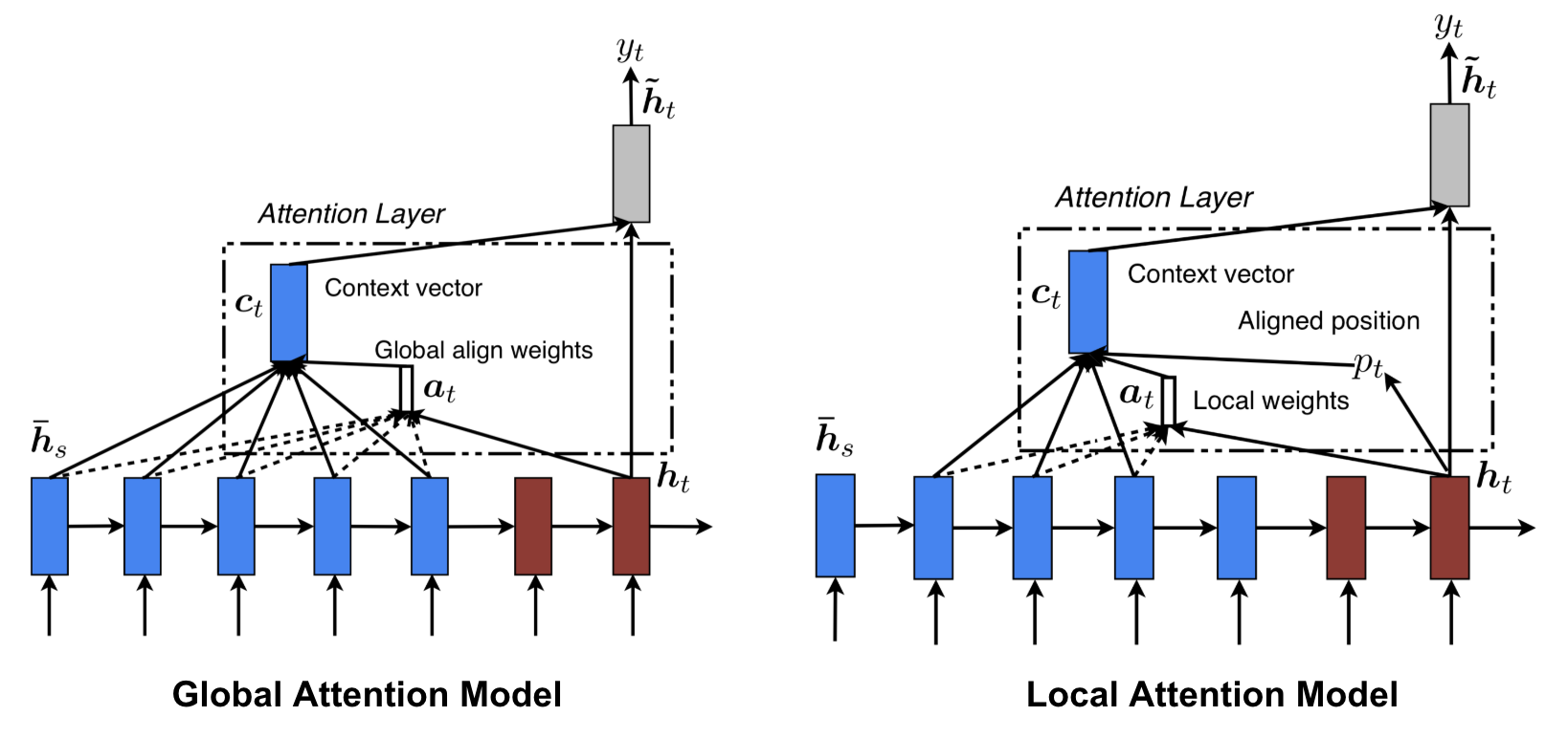
Figure 6. Global vs Local Attention [7] -
Self-attention [10, 13]: attention is placed on different position of same sentence to learn the correlation between the current words and the previous part of the sentence. This will be introduced in more details in next post.
Reference
[1] Visualization of Neural Machine Translation Model
[2] Sutskever, Ilya, Oriol Vinyals, and Quoc V. Le. “Sequence to sequence learning with neural networks.” Advances in neural information processing systems. 2014.
[3] Understanding LSTM Networks
[4] Cho, Kyunghyun, et al. “Learning phrase representations using RNN encoder-decoder for statistical machine translation.” arXiv preprint arXiv:1406.1078 (2014).
[5] Bahdanau, Dzmitry, Kyunghyun Cho, and Yoshua Bengio. “Neural machine translation by jointly learning to align and translate.” arXiv preprint arXiv:1409.0473 (2014).
[7] Luong, Minh-Thang, Hieu Pham, and Christopher D. Manning. “Effective approaches to attention-based neural machine translation.” arXiv preprint arXiv:1508.04025 (2015).
[8] Stanford CS224N: NLP with Deep Learning, Winter 2019, Lecture 8 – Translation, Seq2Seq, Attention
[10] Cheng, Jianpeng, Li Dong, and Mirella Lapata. “Long short-term memory-networks for machine reading.” arXiv preprint arXiv:1601.06733 (2016).
[11] Xu, Kelvin, et al. “Show, attend and tell: Neural image caption generation with visual attention.” International conference on machine learning. 2015.
[12] Gregor, Karol, et al. “Draw: A recurrent neural network for image generation.” arXiv preprint arXiv:1502.04623 (2015).
[13] Vaswani, Ashish, et al. “Attention is all you need.” Advances in neural information processing systems. 2017.