Attention Mechanism [3]: Memory Networks
This is my third note on attention mechanism in deep learning. In this post, I will focus on the memory networks.
Neural Turing Machine: Attention + Memory
Neural Turing Machine (NTM) is proposed in [1] to mimic the Turing Machine by coupling the neural network to external memory resources. Psychologist and neuroscientists have studied working memory process for a long time. Unlike the previous existing work employed the memory mechanism, such as vanilla RNN and LSTM, which only utilize hidden states (internal memory) for memorization that may lose information. NTM represents the external memory as a $N \times M $ matrix, which could be read from and wrote into selectively using self-attention mechanism.
 |
|---|
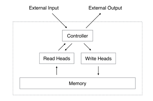
| Figure 1. Neural Turing Machine Architecture. |
As you can see in Figure 1., a NTM contains two components:
-
a memory bank $\mathbf{M}_t$, which is represented by a $N\times M$ matrix over time, where $N$ is the number of memory locations, and $M$ is the vector size at each location.
-
a neural network controller, which could be any neural network architecture.
In addition to interacting to external input and output, the controller will also interact with the memory matrix using a set of parallel selective read and write operations. The selective “blurry” is determined by the well-known attention distribution on the memory matrix.
Reading
For each read head, the reading process will read a vector $\mathbf{r}_t$ from the memory $\mathbf{M}_t$ with selective weight $w_t(i)$ on each memory location
\[\mathbf{r}_t \leftarrow \sum_{i}^{N} w_t(i) \mathbf{M}_t(i)\]where $w_t(i)$ is the $i$-th element in $\mathbf{w}_t$ and $\mathbf{M}_t(i)$ is the $i$-th row vector in the memory, and
\[\sum_{i} w_{t}(i)=1, \quad 0 \leq w_{t}(i) \leq 1, \forall i\]which could be understood as the usual attention distribution. The read process is differentiable because of the convex combination of the row vector $\mathbf{M}_t(i)$ .
Writing
For each write head, the writing process contains two steps: erasing step and adding step. When writing into the memory at time $t$, a write head first wipes off some old content according to an erase vector $\mathbf{e}_t \in (0,1)^M$ and then adds new information by an add vector $\mathbf{a}_t$:
\[\begin{align} \tilde{\mathbf{M}}_{t}(i) &=\mathbf{M}_{t-1}(i)\odot \left[\mathbf{1}-w_{t}(i) \mathbf{e}_{t}\right] \\ \mathbf{M}_{t}(i) &=\tilde{\mathbf{M}}_{t}(i)+w_{t}(i) \mathbf{a}_{t} \end{align}\]where the first equation is erasing step, the second is adding step, and $\odot$ denotes the element-wise multiplication. Since we cannot perform reading and writing at the same time, we can use the same addressing vector $\mathbf{w}_t$ for both operations.
There are something worthing noting:
-
Erase step should be performed before add step
- Since we use multiple heads for writing, the order in which the adds are performed by multiple heads is irrelevant.
- Since both erase and add are differentiable, the composite write operation is differentiable too.
How to obtain the $\mathbf{e}_t$ and $\mathbf{a}_t$ ?
Addressing Mechanisms
The remaining question is where does the attention distribution $\mathbf{w}_t$ come from ? The attention distribution will be derived from two concurrent addressing mechanisms: content-based addressing and location based addressing.
How is addressing being used? For example, we want to perform a copy task tests whether NTM can store and recall a long sequence of arbitrary information. The input is an arbitrary sequence of random binary vectors followed by a delimiter flag. The write process will write the input sequence into the memory matrix beginning with the first input to the last input by modifying the initial memory matrix from $\mathbf{M}_1$ to $\mathbf{M}_T$ . For example, for addressing in this copy task, typically we would like the addressing vector be like $\mathbf{w}_1 = [1, 0, 0, \cdots]$ and write first input into $\mathbf{M}_1(1)$ and the addressing vector $\mathbf{w}_2 = [0,1,0,\cdots]$ and write the second input into $\mathbf{M}_2(2)$ (or next row of first input in memory matrix). To ensure $\mathbf{w}_2$ is a rotational shift of $\mathbf{w}_1$, we need to use the location-based addressing. Once we write the whole input sequence into memory matrix and start the reading step, the machine will use the content-based addressing to find the first stored input and location-based addressing to read the next stored input. The target output is simply a copy of the input sequence (without the delimiter flag).
Content-based Addressing
\[w_{t}^{c}(i) \longleftarrow \frac{\exp \left(\beta_{t} K\left[\mathbf{k}_{t}, \mathbf{M}_{t}(i)\right]\right)}{\sum_{j} \exp \left(\beta_{t} K\left[\mathbf{k}_{t}, \mathbf{M}_{t}(j)\right]\right)}\]where $\beta_t$ is a positive key strength, which can amplify or attenuate the precision of the focus, $\mathbf{k}_t$ is a length $M$ key vector produced by each head, and $K[\cdot, \cdot]$ is a similarity measure. Note that key vectors will be learned via training.
Location-based Addressing
The location based addressing mechanism is designed to facilitate both simple iteration across the locations of the memory and random-access jumps. It does so by implementing a rotational shift of a weighting [1]. Think about the situation that we would like $\mathbf{w}_{t-1} = [1, 0, 0, \cdots]$ becomes $\mathbf{w}_t = [0, 1, 0, 0, \cdots ]$, how could be achieve this ?
Gated Weighting: we need to consider both (or either one of) the content system at the current time-step $\mathbf{w}_t^{c}$ and the location system at the previous time-step $\mathbf{w}_{t-1}$:
\[\mathbf{w}_{t}^{g} \longleftarrow g_{t} \mathbf{w}_{t}^{c}+\left(1-g_{t}\right) \mathbf{w}_{t-1}\]where $g_t \in (0,1)$ can be viewed as interpolation gate which is emit by each head.
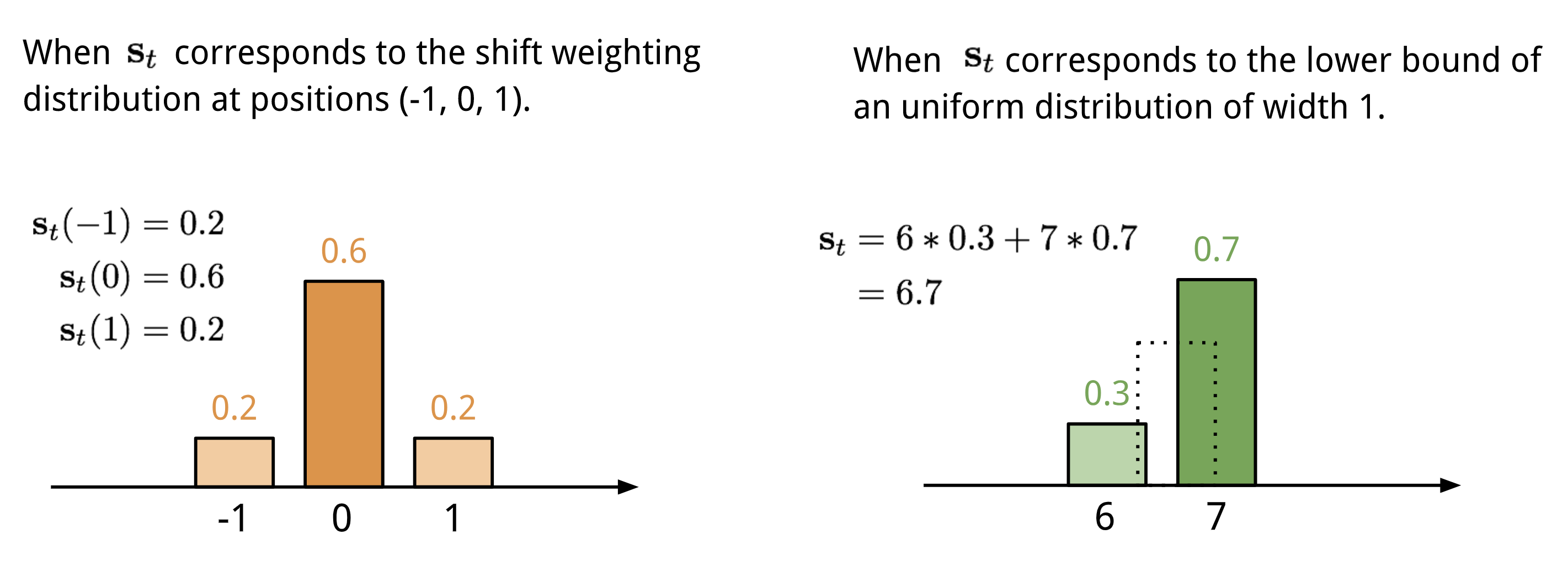
Shift Weighting: After interpolation (or gated weighting), each head emits a shift weighting $\mathbf{s}_t$ that defines a normalized distribution over the allowed integer shifts. For example, let $\mathbf{w}_{t-1} = [1, 0, 0]$ and $g_t = 0$, if we would like the system shifts the focus to next memory location, that is $\mathbf{w}_t = [0,1,0]$, how can we do that ? Recall the image shifting in CNN, we could also apply 1-D circular convolution, where $\mathbf{s}_t$ is the filter, a function of the position offset:
\[\tilde{w}_{t}(i) \longleftarrow \sum_{j=0}^{N-1} w_{t}^{g}(j) s_{t}(i-j)\]There are multiple ways to define the shift weighting distribution [3]:
 |
|---|
| Figure 2. Two ways to represent the shift weighting distribution $\mathbf{s}_t$ (Explanation from [3]). |
In addition, we need to sharpen the final weighting to avoid blurred shifting:
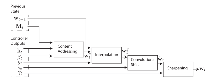
\[w_{t}(i) \longleftarrow \frac{\tilde{w}_{t}(i)^{\gamma_{t}}}{\sum_{j} \tilde{w}_{t}(j)^{\gamma_{t}}}\]In summary, the flow diagram shows the overall addressing mechanism:
 |
|---|
| Figure 3. Flow Diagram of the Addressing Mechanism [1] |
Dynamic Key-value Memory Networks
Knowledge Tracing Problem: given a student’s past exercise interaction \(\mathcal{X} = \{\mathbf{x}_1, \cdots, \mathbf{x}_{t-1}\}\), where \(\mathbf{x}_i = (q_i, r_i)\), predicts the probability that the student will answer a new exercise correctly, i.e. \(p(r_t = 1 \mid q_t, \mathcal{X})\), where \(q_i \in Q\) and \(r_i \in \{0, 1\}\).
Dynamic Key-value Memory Networks (DKVMN) is a variant of Memory-Augmented Neural Networks. It is proposed to not only handle the knowledge tracing task but also exploit the relationship between underlying concepts and directly output a student’s mastery level of each concept. It leverages the augmented memory neural network with static matrix for storing the knowledge concept and dynamic matrix for storing and updating the mastery levels of corresponding concepts. The storing and updating processes utilize the self-attention mechanism.
Potential Way to Address Knowledge Tracing with MANN
The advantages of MANN over the internal memory architecture, such as DKT with LSTM:
- DKT with LSTM uses a single hidden state vector to encode the temporal information, whereas, MANN uses an external memory matrix that can increase storage capacity.
- the state-to-state transition of traditional RNNs is unstructured and global, whereas MANN uses read and write operations to encourage local state transitions.
- the number of parameters in traditional RNNs is tied to the size of hidden states.
 |
|---|
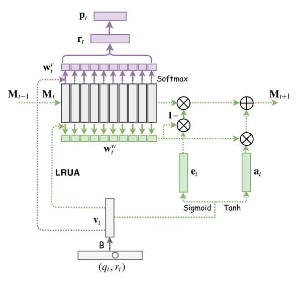
| Figure 4. Architecture for Memory-Augmented Neural Networks |
As you can see in Figure 4., the input of MANN is a joint embedding $\mathbf{v}_t$ of $(q_t, r_t)$, which will be used to compute the read weight $\mathbf{w}_t^r$ with content-based addressing and the write weight $\mathbf{w}_t^{w}$ with LRUA mechanism. The purple components describe the read process and the green component describe the write process. But, wait, something is wrong:
- when we make the prediction, the input is just question $q_t$ without response $r_t$, and thus the input embedding $\mathbf{v}_t$ will not be accurate and further result in inaccurate reading process and prediction.
- MANN cannot explicitly model the underlying concepts for input exercise.
DKVMN: Address the Limitations of MANN on KT.
 |
|---|
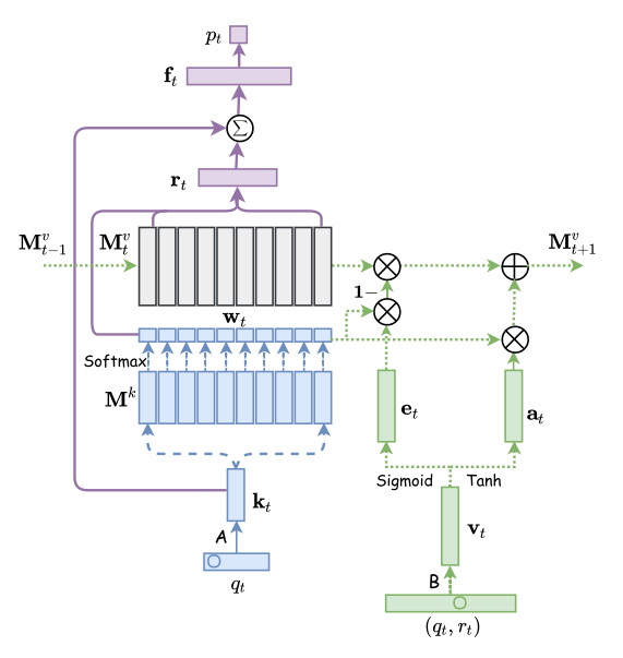
| Figure 5. DKVMN Architecture. |
As you can see in the figure 5, the input of DKVMN is still $(q_t, r_t)$, but it will separately generate embeddings $\mathbf{k}_t$ (purely based on $q_t$) and $\mathbf{v}_t$ (based on ($q_t, r_t$ )). In order to model the underlying concepts of each exercise, DKVMN utilizes a static matrix $\mathbf{M}^k \in \mathbb{R}^{N \times d_k}$ (key matrix) to represent the $N$ latent concepts\(\{c^1, c^2, \cdots, c^N \}\), each of which is represented by $d_k$ dimensional vector. In order to tracing student’s mastery levels of each concept, DKVMN employs a matrix $\mathbf{M}^{v}_t \in \mathbb{R}^{N \times d_v}$ (value matrix) to store concept states \(\{\mathbf{s}_t^1, \mathbf{s}_t^2, \cdots, \mathbf{s}_t^N \}\) at time $t$ .
Reading
The intuition is, when we want to predict a student’s performance on exercise $q_t$, we need to find the correlation between the exercise $q_t$ and the $N$ latent concepts. Similar to the content-based addressing in Neural Turing Machine, we could compute the correlation by
\[w_{t}(i) \longleftarrow \frac{\exp \left( \mathbf{k}_{t}^\top \mathbf{M}_{t}(i)\right)}{\sum_{j} \exp \left(\mathbf{k}_{t}^\top \mathbf{M}_{t}(j)\right)}\]then we could use this concept correlation weight to retrieve the student’s mastery level of this exercise by attending $\mathbf{M}^{v}_{t}$ (student’s knowledge state at current time $t$) :
\[\mathbf{r}_{t}=\sum_{i=1}^{N} w_{t}(i) \mathbf{M}_{t}^{v}(i)\]Then, $\mathbf{r}_t$ (student’s mastery level of this exercise at time $t$) will be employed to obtain the final output, the probability of answering $q_t$ correctly, via
\[\mathbf{f}_{t}=\tanh \left(\mathbf{W}_{1}^{T}\left[\mathbf{r}_{t}, \mathbf{k}_{t}\right]+\mathbf{b}_{1}\right)\]\(p_{t}=\operatorname{Sigmoid}\left(\mathbf{W}_{2}^{T} \mathbf{f}_{t}+\mathbf{b}_{2}\right)\) The reason to concatenate the $\mathbf{r}_t$ with $\mathbf{k}_t$ is that it is better to contain “both the student’s mastery level and the prior difficulty of the exercise” to make prediction. But, I think $\mathbf{r}_t$ has already contained the student’s mastery level w.r.t this exercise at time, and the exercise difficulty may not be useful ?
Writing
The writing process will update student’s knowledge state $\mathbf{M}^v_t$ based on $(q_t, r_t)$. The intuition is, if student answers the question correctly, we would like to update the $\mathbf{M}_t^v$ based on the correlation between question and concepts, that is $\mathbf{w}_t$. The $\mathbf{v}_t \in \mathbb{R}^{2Q\times d_v}$joint embedding of $(q_t, r_t)$ could be viewed as the knowledge gain of the student after working on this exercise.
Inspired by the NTM, knowledge updating step contains two steps: erase step and add step:
\(\begin{align} \tilde{\mathbf{M}}_{t}^{v}(i)&=\mathbf{M}_{t-1}^{v}(i)\odot\left[\mathbf{1}-w_{t}(i) \mathbf{e}_{t}\right] \\ \mathbf{M}_{t}^{v}(i)&=\tilde{\mathbf{M}}_{t-1}^{v}(i)+w_{t}(i) \mathbf{a}_{t} \end{align}\) where $\mathbf{e}_t$ and $\mathbf{a}_t$ could be computed from the knowledge gain vector $\mathbf{v}_t$
\[\begin{align} \mathbf{e}_{t}&=\operatorname{Sigmoid}\left(\mathbf{E}^{T} \mathbf{v}_{t}+\mathbf{b}_{e}\right) \\ \mathbf{a}_{t}&=\operatorname{Tanh}\left(\mathbf{D}^{T} \mathbf{v}_{t}+\mathbf{b}_{a}\right) \end{align}\]Reference
[1] Graves, Alex, Greg Wayne, and Ivo Danihelka. “Neural turing machines.” arXiv preprint arXiv:1410.5401 (2014).
[2] Neural Turing Machine - ZhiHu
[4] Santoro, Adam, et al. “Meta-learning with memory-augmented neural networks.” International conference on machine learning. 2016.
[5] Zhang, Jiani, et al. “Dynamic key-value memory networks for knowledge tracing.” Proceedings of the 26th international conference on World Wide Web. 2017.