Top-k Off-Policy Correction for a REINFORCE Recommender System

This is a paper from Google published in WSDM-2019 conference on applying reinforcement learning on industry-level recommender system in Youtube.

• Motivation
• Contributions
• Proposed Methods
  • REINFORCE Recommender
    • Objective
    • REINFORCE: a policy-gradient-based approach
    • Off-Policy Correction
  • Parametrising the Policy $\pi_{\theta}$
  • Estimating the Behavior Policy $\beta$
  • Top-k Off-Policy Correction
  • Variance Reduction Techniques
  • Exploration
• Reference

Motivation

• There are a lot logged feedback from customers in recommender system, but subject to system biases caused by only observing feedback on recommendations selected by the previous versions of the recommender.
• It is difficult to apply reinforcement learning on recommender systems, because:
  1. it deals with large state and action spaces.
  2. the set of items available to recommend is non-stationary and new items are brought into the system constantly, resulting in an ever-growing action space with new items having even sparser feedback.
  3. user preferences over these items are shifting all the time, resulting in continuously-evolving user states
• Classic RL could use self-play and simulation to collect training data, but not suitable for recommender systems. Therefore, the model has to relies mostly on data made available from the previous recommendation models (policies), most of which we cannot control or can no longer control.
• There are some existing methods to reduce system biases on off-policy evaluation with reinforcement learning. But there is no existing method on the problem of off-policy training of top-k items recommendation with reinforcement learning.

Contributions

• Scale a REINFORCE policy-gradient-based approach to learn a neural recommendation policy in a extremely large action space.
• Apply off-policy correction to learn from logged feedback, collected from an ensemble of prior model policies.
• Define a novel top-k off-policy correction for top-k recommender system.
• An real-world RL application and live experiments demonstration.

Proposed Methods

REINFORCE Recommender

The Markov Decision Process (MDP) is $(\mathcal{S}, \mathcal{A}, \mathbf{P}, R, \rho_0, \gamma)$:

• $\mathcal{S}$: a continuous state space describing the user states, which could be user’s preference;
• $\mathcal{A}$: a discrete action space, containing items available for recommendation;
• $\mathbf{P}: \mathcal{S}\times\mathcal{A}\times\mathcal{S}\rightarrow \mathbb{R}$ is the state transition probability;
• $R: \mathcal{S}\times \mathcal{A}\rightarrow \mathbb{R}$ is the reward function, where $r(s, a)$ is the immediate reward obtained by performing action a at user state $s$;
• $\rho_0$ is the initial state distribution;
• $\gamma$ is the discount factor for future rewards.

Objective

The expected cumulative reward is:

\[J(\theta) = \mathbb{E}_{\tau \sim \pi_{\theta}}[R(\tau)]\quad \text { where } \quad R(\tau)=\sum_{t=0}^{|\tau|} r\left(s_{t}, a_{t}\right)\]

where assuming policy $\pi_{\theta}(a\mid s)$ is a function parameterized by $\theta\in\mathbb{R}^d$, and the expectation is taken over the trajectories

\[\tau = (s_0, a_0, s_1, \cdots)\]

obtained by acting according to the policy:

\[\begin{align} s_0 &\sim \rho_0, \\ a_t &\sim \pi(\cdot, s_t), \\ s_{t+1} &\sim \mathbf{P}(\cdot\mid s_t, a_t) \end{align}\]

For example, in episodic tasks, the probability of occurrence of one specific episode $\tau$ under policy $\pi$ is:

\[p_{\theta}(\tau) =p_{\theta}\left(s_{0}, a_{0}, \cdots, s_{T}, a_{T}\right) =p\left(s_{0}\right) \prod_{t}\left[\pi_{\theta}\left(a_{t} | s_{t}\right) \cdot p\left(s_{t+1} | s_{t}, a_{t}\right)\right]\]

where $\rho_0 = p(s_0)$. The objective is to find a policy $\pi_{\theta}$ that maximizes the expected cumulative reward obtained by the recommender system:

\[\max _{\theta} J(\theta)\]

REINFORCE: a policy-gradient-based approach

The most straightforward way is to maximize the expected cumulative reward via gradient descent w.r.t $\color{blue}{\theta}$ . Hence, we need to derive the $\nabla_{\color{blue}{\theta}} J(\theta)$, that is

\[\begin{align} \nabla_{\theta} J(\theta) &= \sum_{\tau} R(\tau) \nabla_{\theta} p_{\theta}(\tau) \\ &= \sum_{\tau} R(\tau) \color{blue}{p_{\theta}(\tau) \frac{\nabla_{\theta} p_{\theta}(\tau)}{p_{\theta}(\tau)}} \\ &= \sum_{\tau} R(\tau) \color{blue}{p_{\theta}(\tau) \nabla_{\theta} \log p_{\theta}(\tau)}\\ &= \color{red}{\operatorname{E}_{\tau \sim p_{\theta}(\tau)} \left[ R(\tau) \nabla_{\theta} \log p_{\theta}(\tau) \right]} \\ &\color{red}{\approx} \frac{1}{N} \sum_{n=1}^{N} R(\tau^n) \nabla_{\theta} \log p_{\theta}(\tau^n) \\ &= \frac{1}{N} \sum_{n=1}^{N} R(\tau^n) \nabla_{\theta} \log \left\{ p\left(s_{0}^{n} \right) \prod_{t}\left[\pi_{\theta}\left(a_{t}^{n} | s_{t}^{n}\right) \cdot p\left(s_{t+1}^{n} | s_{t}^{n}, a_{t}^{n}\right)\right]\right\} \\ &= \frac{1}{N} \sum_{n=1}^{N} R(\tau^n) \nabla_{\theta} \log \left[ \prod_{t}\pi_{\theta}\left(a_{t}^{n} | s_{t}^{n}\right) \right] \\ &= \frac{1}{N} \sum_{n=1}^{N} R(\tau^n) \sum_{t=0} \nabla_{\theta} \log \pi_{\theta}\left(a_{t}^{n} | s_{t}^{n} \right) \\ &=\frac{1}{N} \sum_{n=1}^{N} \left[ \sum_{t=0}^{|\tau^n|} r(s_t, a_t) \right] \left[\sum_{t=0}^{|\tau^n|} \nabla_{\theta} \log \pi_{\theta}\left(a_{t}^{n} | s_{t}^{n}\right) \right] \\ &=\frac{1}{N} \sum_{n=1}^{N} \left[ \sum_{t=0}^{|\tau^n|} \left( \sum_{t=0}^{|\tau^n|} r(s_t, a_t) \right) \nabla_{\theta} \log \pi_{\theta}\left(a_{t}^{n} | s_{t}^{n}\right) \right] \end{align}\]

    
\begin{algorithm}
\caption{REINFORCE}
\begin{algorithmic}
\STATE sample $\left\{\tau^{n}\right\}$ from $\pi_{\theta}\left(a_{t} \mid s_{t}\right)$ (run the policy)
\STATE $\nabla_{\theta} J(\theta) \approx \frac{1}{N} \sum_{n}^{N}\left[\sum_{t} \left(\sum_{t} r\left(\mathbf{s}_{t}^{n}, \mathbf{a}_{t}^{n}\right)\right) \nabla_{\theta} \log \pi_{\theta}\left(\mathbf{a}_{t}^{n} \mid \mathbf{s}_{t}^{n}\right)\right]$
\STATE $\theta \leftarrow \theta+\alpha \nabla_{\theta} J(\theta)$
\end{algorithmic}
\end{algorithm}

In addition, we could replace $\color{red}{ \left( \sum_{t=0}^{\vert \tau^{n} \vert } r(s_t, a_t) \right) }$ with a discounted future reward $ R_t = \sum_{t’=t}^{\vert \tau^{n} \vert} \gamma^{(t’-t)} r(s_{t’}, a_{t’}) $ for action at time $t$ to reduce variance in the gradient estimate.

Off-Policy Correction

Policy gradient, for example REINFORCE algorithm, is an on-policy method. It is inefficient to iteratively update the model $ \pi_{\theta} $ and then generate new trajectories. Off-policy method is to train the policy $\pi_{\theta}$, called target policy, by using the sampled trajectories generated by another policy $ \pi_{\omega}$, called behavior policy. In this way, we can reuse the sample trajectories.

Off-policy method has different form of objective function:

\[J(\theta) = \mathbf{E}_{\tau \sim p_{\theta}(\tau)} \left[R(\tau) \right] = \mathbf{E}_{\tau \sim \color{red}{p_{\omega}(\tau)}}\left[\frac{p_{\theta}(\tau)}{p_{\omega}(\tau)} R(\tau)\right]\]

which leverages the important sampling

\[\begin{align} E_{x \sim p(x)}[f(x)] &=\int p(x) f(x) d x \\ &=\int \frac{q(x)}{q(x)} p(x) f(x) d x \\ &=\int q(x) \frac{p(x)}{q(x)} f(x) d x \\ &=E_{x \sim q(x)}\left[\frac{p(x)}{q(x)} f(x)\right] \end{align}\]

We can compute the ratio $ \frac{p_{\theta}(\tau)}{p_{\omega}(\tau)}$ which is known as importance weight

\[\begin{align} \frac{p_{\theta}(\tau)}{p_{\omega}(\tau)} &=\frac{\rho_{\theta}\left(s_{0}\right) \prod_{t=0}^{|\tau|} \pi_{\theta}\left(a_{t} | s_{t}\right) \rho_{\theta}\left(s_{t+1} | s_{t}, a_{t}\right)}{ \rho_{\omega}\left(s_{0}\right) \prod_{t=0}^{|\tau|} \pi_{\omega}\left(a_{t} | s_{t}\right) \rho_{\omega}\left(s_{t+1} | s_{t}, a_{t}\right)}\\ &=\frac{ \prod_{t=0}^{|\tau|} \pi_{\theta}\left(a_{t} | s_{t}\right)}{\prod_{t=0}^{|\tau|} \pi_{\omega}\left(a_{t} | s_{t}\right)} \end{align}\]

where we use the fact that different policies do not effect the transition probabilities of the environment, that is $ p_{\theta}(s_{0}) = p_{\omega}(s_{0}) $. However, the variance of the estimator is huge due to the chained products, leading quickly to very low or high values of the importance weights. In addition, this will also lead to gradient vanishing or exploding in RNNs. Two approaches are used to reduce the variance:

1. ignore the terms after time $t$.
2. first-order approximation.

Therefore,

\[\begin{align} \prod_{t'=0}^{|\tau|} \frac{\pi_{\theta}\left(a_{t'} | s_{t'}\right)}{ \pi_{\omega}\left(a_{t'} | s_{t'}\right)} \approx \prod_{t'=0}^{\color{red}{t}} \frac{\pi_{\theta}\left(a_{t'} | s_{t'}\right)}{ \pi_{\omega}\left(a_{t'} | s_{t'}\right)} = \frac{p_{\pi_{\theta}}(s_t)}{p_{\pi_{\omega}}(s_t)} \frac{\pi_{\theta}\left(a_{t} | s_{t}\right)}{ \pi_{\omega}\left(a_{t} | s_{t}\right)} \approx \frac{\pi_{\theta}\left(a_{t} | s_{t}\right)}{ \pi_{\omega}\left(a_{t} | s_{t}\right)} \end{align}\]

where $p_{\pi_{\theta}}(s_t)$ represents the probability of state $s_t$ under policy $\pi_{\theta}$. Therefore, we can derive a biased estimator of the policy gradient w.r.t parameter $\theta$ with lower variance as:

\[\begin{align} \nabla_{\theta} J(\theta) &= \mathbf{E}_{\tau \sim p_{\omega}(\tau)} \left[ \frac{\nabla p_{\theta}(\tau) }{p_{\omega}(\tau)} R(\tau)\right] \\ &= \mathbf{E}_{\tau \sim p_{\omega}(\tau)} \left[ \frac{p_{\theta}(\tau) \nabla \log p_{\theta}(\tau)}{p_{\omega}(\tau)} R(\tau)\right] \\ &= \mathbf{E}_{\tau \sim p_{\omega}(\tau)} \left[ \frac{p_{\theta}(\tau) }{p_{\omega}(\tau)} \nabla \log p_{\theta}(\tau) R(\tau)\right] \\ &= \mathbf{E}_{\tau \sim p_{\omega}(\tau)}\left[\left(\prod_{t=0}^{|\tau|} \frac{\pi_{\theta} \left(a_{t} | s_{t}\right)}{\pi_{\omega}\left(a_{t} | s_{t}\right)}\right)\left(\sum_{t=0}^{|\tau|} \nabla_{\theta} \log \pi_{\theta} \left(a_{t} | s_{t}\right)\right)\left(\sum_{t=0}^{|\tau|} r\left(s_{t}, a_{t}\right)\right)\right]\\ &\approx \mathbf{E}_{\tau \sim p_{\omega}(\tau)}\left[\frac{\pi_{\theta} \left(a_{t} | s_{t}\right)}{\pi_{\omega}\left(a_{t} | s_{t}\right)}\left(\sum_{t=0}^{|\tau|} \nabla_{\theta} \log \pi_{\theta} \left(a_{t} | s_{t}\right)\right)R_t\right]\\ &\approx \frac{1}{N} \sum_{\tau \sim \pi_{\omega}}\left[\sum_{t=0}^{|\tau|} \frac{\pi_{\theta} \left(a_{t} | s_{t}\right)}{\pi_{\omega}\left(a_{t} | s_{t}\right)} R_t \nabla_{\theta} \log \pi_{\theta} \left(a_{t} | s_{t}\right)\right] \end{align}\]

Parametrising the Policy $\pi_{\theta}$

• $\mathbf{s}_t \in \mathbb{R}^n$ denotes by user interests at time $t$.

• $\mathbf{u}_{a_t} \in \mathbb{R}^m$ denotes by action taken at time $t$.

• The state transition (or user interest transition modeling) $\mathbf{P}: \mathcal{S}\times \mathcal{A} \times \mathcal{S}$ is modeled by a Chaos Free RNN (CFN):

  \[\mathbf{s}_{t+1} = f(\mathbf{s}_t, \mathbf{u}_{a_t})\]

  where the state is updated recursively as

  \[\begin{aligned} \mathbf{s}_{t+1} &=\mathbf{z}_{t} \odot \tanh \left(\mathbf{s}_{t}\right)+\mathbf{i}_{t} \odot \tanh \left(\mathbf{W}_{a} \mathbf{u}_{a_{t}}\right) \\ \mathbf{z}_{t} &=\sigma\left(\mathbf{U}_{z} \mathbf{s}_{t}+\mathbf{W}_{z} \mathbf{u}_{a_{t}}+\mathbf{b}_{z}\right) \\ \mathbf{i}_{t} &=\sigma\left(\mathbf{U}_{i} \mathbf{s}_{t}+\mathbf{W}_{i} \mathbf{u}_{a_{t}}+\mathbf{b}_{i}\right) \end{aligned}\]

  where $\mathbf{z}_t, \mathbf{i}_t \in \mathbb{R}^n$ are the update and input gate respectively.

• Conditioning on a user state s, the policy $\pi_{\theta} (a\mid s)$ is then modeled with softmax:

  \[\pi_{\theta}(a \mid \mathbf{s})=\frac{\exp \left(\mathbf{s}^{\top} \mathbf{v}_{a} / T\right)}{\sum_{a^{\prime} \in \mathcal{A}} \exp \left(\mathbf{s}^{\top} \mathbf{v}_{a^{\prime}} / T\right)}\]

• • $\mathbf{v}_a \in \mathbb{R}^n$ is another embedding for each action $a$.

  • $T$ is a temperature that is normally set to 1.
  • If $\vert \mathcal{A} \vert$ is very large, we could use sampled softmax.

• The parameter $\theta$ of the policy $\pi_{\theta}$ contains:

  • two action embeddings $\mathbf{U} \in \mathbb{R}^{m \times \vert\mathcal{A} \vert}$ and $\mathbf{V} \in \mathbb{R}^{n \times \vert\mathcal{A}\vert}$.
  • weight matrices $\mathbf{U}_z, \mathbf{U_i}\in \mathbb{R}^{n\times n}$.
  • weight matrices $\mathbf{W}_{z}, \mathbf{W}_i, \mathbf{W}_a \in \mathbb{R}^{n \times m}$.
  • biases $\mathbf{b}_z, \mathbf{b}_i \in \mathbf{R}^n$.

• Architecture Diagram:

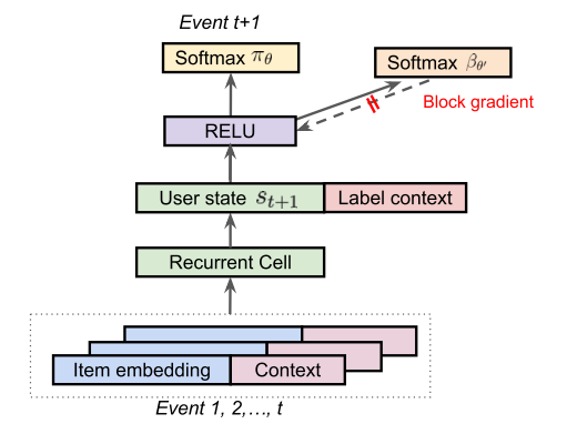
  policy $\pi_{\theta}$ architecture.

  • Given an observed trajectory $\tau = (s_0, a_0, s_1, \cdots)$ sampled from a behavior policy $\beta$.

  • The new policy firstly generate the initial state $\mathbf{s}_0 \sim \rho_0$.

  • Iterate through the recurrent cell to get the user state $\mathbf{s}_{t+1}$.

  • With $\mathbf{s}_{t+1},$ we are able to get the $\pi_{\theta}(a_{t+1} \mid \mathbf{s}_{t+1})$ distribution.

  • With $\pi_{\theta}(a_{t+1} \mid \mathbf{s}_{t+1})$, we are able to produce a policy gradient to update the policy.

  • $\pi_{\theta}$ is trained using only items on the trajectory with non-zero reward, since actions with zero-reward will not contribute to the gradient update in $\pi_{\theta}$.

Estimating the Behavior Policy $\beta$

• The policy gradient estimation formula contains the behavior policy in the denominator. But we don’t have controls over behavior policy, we have to estimate it.

• Behavior policy in this paper is a mixture of the policies.

• For each state-action pair $(s, a)$ collected, it estimates the probability $\hat{\beta}_{\theta’}(a\mid s)$ that the mixture of behavior policies choosing that action using another softmax, parameterised by $\theta’$.

• User state representation is re-used, as you can see in the aechitecture diagram.

• $\theta’$ is trained like supervised learning with logged state-action pairs, and the behavior head should not intefering with the user state of the main policy, as you can see the block gradient in the figure.

• If the behavior policy is deterministic with different actions at different time, then we should treat it as randomization among actions.

Top-k Off-Policy Correction

• In classic reinforcement learning, user interacts with one item. But in recommender system, we need to pick a set of relevant items instead of a single one.

• We seek a policy $\Pi_{\Theta}(A \mid s)$, here each action $A$ is to select a set of $k$ items, to maximize the expected cumulative reward,

  \[\max _{\Theta} \mathbb{E}_{\tau \sim \Pi_{\theta}}\left[\sum_{t} r\left(s_{t}, A_{t}\right)\right]\]
• \[\begin{align} \tau &\sim (s_0, A_0, s_1, \cdots) \\ s_0 &\sim \rho_0\\ A_t &\sim \Pi(\cdot\mid s_t)\\ s_{t+1} &\sim \mathbf{P}(\cdot\mid s_t, A_t) \end{align}\]

• Assume the expected reward of a set of non-repetitive items equal to the sum of the expected reward of each item in the set.

• Generate the set action $A$ by independently sampling each item $a$ according to the softmax policy $\pi_{\theta}$ and then de-duplicate. That is,

  \[\Pi_{\Theta}\left(A^{\prime} \mid s\right)=\prod_{a \in A^{\prime}} \pi_{\theta}(a \mid s)\]

• Modify the on-policy gradient update:

  \[\frac{1}{N} \sum_{\color{red}{\tau\sim \pi_{\theta}}} \left[\sum_{t=0}^{|\tau|} R_{t} \nabla_{\theta} \log \alpha_{\theta}\left(a_{t} \mid s_{t}\right)\right]\]

  where

  \[\color{blue}{\alpha_{\theta}(a\mid s) = 1- (1-\pi_{\theta}(a\mid s))^K}\]

  is the probability that an item $a$ appears in the final non-repetitive set $A$.

• Replace $\pi_{\theta}$ with $\alpha_{\theta}$ and apply log-trick to get the top-K off-policy corrected gradient:

  \[\begin{align} &\quad \ \frac{1}{N} \sum_{\color{red}{\tau\sim \beta}}\left[\sum_{t=0}^{|\tau|} \frac{\alpha_{\theta} \left(a_{t} | s_{t}\right)}{\beta\left(a_{t} | s_{t}\right)} R_t \nabla_{\theta} \log \alpha_{\theta} \left(a_{t} | s_{t}\right)\right]\\ &= \frac{1}{N} \sum_{\tau \sim \beta}\left[\sum_{t=0}^{|\tau|} \frac{\alpha_{\theta}\left(a_{t} \mid s_{t}\right)}{\beta\left(a_{t} \mid s_{t}\right)} R_{t} \frac{\nabla_{\theta}\alpha_{\theta}(a_t\mid s_t)}{\alpha_{\theta}(a_t\mid s_t)}\right]\\ &= \frac{1}{N} \sum_{\tau \sim \beta}\left[\sum_{t=0}^{|\tau|} \frac{\alpha_{\theta}\left(a_{t} \mid s_{t}\right)}{\beta\left(a_{t} \mid s_{t}\right)} R_{t} \frac{\partial\alpha(a_t \mid s_t)}{\partial \pi(a_t, s_t)}\cdot \frac{\partial \pi_{\theta}(a_t\mid s_t)}{\alpha_{\theta}(a_t\mid s_t)} \right]\\ &= \frac{1}{N} \sum_{\tau \sim \beta}\left[\sum_{t=0}^{|\tau|} \frac{\color{red}{ {\alpha_ {\theta} \left(a_{t} \mid s_{t}\right)}} \pi_{\theta}(a_t\mid s_t)}{\beta\left(a_{t} \mid s_{t }\right)} R_{t} \frac{\partial\alpha(a_t \mid s_t)}{\partial \pi(a_t, s_t)}\cdot \frac{\partial \pi_{\theta}(a_t\mid s_t)}{\alpha_{\theta}(a_t\mid s_t)}\pi_{\theta}(a_t\mid s_t) \right]\\ &=\frac{1}{N} \sum_{\tau \sim \beta}\left[\sum_{t=0}^{|\tau|} \frac{\pi_{\theta}\left(a_{t} \mid s_{t}\right)}{\beta\left(a_{t} \mid s_{t}\right)} \color{blue}{\frac{\partial \alpha\left(a_{t} \mid s_{t}\right)}{\partial \pi\left(a_{t} \mid s_{t}\right)}} R_{t} \nabla_{\theta} \log \pi_{\theta}\left(a_{t} \mid s_{t}\right)\right] \end{align}\]

• The only difference between previous off-policy corrected gradient and top-k off-policy corrected gradient is the additional multiplier:

  \[\lambda_{K}\left(s_{t}, a_{t}\right)=\frac{\partial \alpha\left(a_{t} \mid s_{t}\right)}{\partial \pi\left(a_{t} \mid s_{t}\right)}=K\left(1-\pi_{\theta}\left(a_{t} \mid s_{t}\right)\right)^{K-1}\]

  • As $\pi_{\theta} (a\mid s) \rightarrow 0,\quad \lambda_K(s, a) \rightarrow K$. If at state $s$ the new policy $\pi$ barely choose action $a$, then we increase the policy update by a factor of $K$ comparing to the standard off-policy correction. When the desirable item has a small mass in the softmax policy $\pi_{\theta} (·\mid s)$, the top-K correction more aggressively pushes up its likelihood than the standard correction.

  • As $\pi_{\theta} (a\mid s) \rightarrow 1,\quad \lambda_K(s, a) \rightarrow 0$. If at state $s$ the new policy $\pi$ always choose action $a$, then we don’t do the policy update. Once the softmax policy $\pi_{\theta} (·\mid s)$ casts a reasonable mass on the desirable item (to ensure it will be likely to appear in the top-K), the correction then zeros out the gradient and no longer tries to push up its likelihood.

  • As K increases, this multiplier reduces the gradient to zero faster as $\pi_{\theta} (a\mid s) $ $\color{red}{\text{reaches a reasonable range?}}$

Variance Reduction Techniques

We need to pay attention to the importance weight:

\[\omega(s, a) = \frac{\pi(a\mid s)}{\beta(a \mid s)}\]

which could be very large due to:

1. $\pi(a\mid s) » \beta(a\mid s)$ when new policy $\pi$ explores regions that are less explored by the behavior policy $\beta$.
2. large variance in the $\beta$ estimate.

There are several approaches to reduce the variance of estimated policy gradient (but introduce some bias):

1. Discounted rewards, because the future rewards are far uncertain than more recent rewards.

2. Ignore the terms after the time $t$ in importance weight, similar to discounted rewards.

3. First order approximation.

4. Weight capping. Smaller value of $c$ reduces variance in the gradient estimate, but introduces larger bias.

   \[\bar{\omega}_{c}(s, a)=\min \left(\frac{\pi(a \mid s)}{\beta(a \mid s)}, c\right)\]

5. Normalized Importance Sampling:

   \[\bar{\omega}_{n}(s, a)=\frac{\omega(s, a)}{\sum_{\left(s^{\prime}, a^{\prime}\right) \sim \beta} \omega\left(s^{\prime}, a^{\prime}\right)}\]

6. Trusted Region Policy Optimization (TRPO). TRPO prevents the new policy $\pi$ from deviating from the behavior policy by adding a regularization that penalizes the KL divergence of these two policies. It achieves similar effect as the weight capping.

Exploration

• Boltzmann exploration.

• Use stochastic policy where recommendations are sampled from $\pi_{\theta}$ rather than taking the $K$ items with the highest probability,

• Compute full softmax over all actions is computational inefficiency.

• Efficient approximate nearest neighbor-based systems to look up the top $M$ items in the softmax.

• Apply softmax on those $M$ items, and sampling $K$ items from those $M$ items.

• Exploitation: $K’$ most probable items. Exploration: $K - K’$ items from the remaining $M-K’$ items.

Reference

[1] Top-k Off-Policy Correction for a REINFORCE Recommender System

[2] Paper Presentation Video

[3] Reinforcement Learning for Slate-based Recommender Systems: A Tractable Decomposition and Practical Methodology